Mapping multiple trends with confidence

We will use dplyr::nest to create a list-column and will apply a model (with purrr::map) to each row, then we will extract each slope and its p value with map and broom::tidy.

Setup

library(tidyverse)
library(httr)
library(sf)
library(readxl)
library(janitor)
library(fs)
library(broom)
library(scales)
library(rnaturalearth)
library(glue)

Data

Map data. Départements polygons from modified Adminexpress

dep <- st_read("~/data/adminexpress/adminexpress_cog_simpl_000_2022.gpkg",
               "departement")

Reading layer `departement' from data source 
  `/home/michael/data/adminexpress/adminexpress_cog_simpl_000_2022.gpkg' 
  using driver `GPKG'
Simple feature collection with 103 features and 4 fields
Geometry type: MULTIPOLYGON
Dimension:     XY
Bounding box:  xmin: -63.15272 ymin: -21.38883 xmax: 55.83661 ymax: 51.08876
Geodetic CRS:  WGS 84

Population data by département from INSEE.

if (!file_exists("pop.xlsx")) {
  GET("https://www.insee.fr/fr/statistiques/fichier/2012713/TCRD_004.xlsx",
      write_disk("pop.xlsx"))
}
  
pop <- read_xlsx("pop.xlsx", skip = 3, na = "nd") |> 
  clean_names() |> 
  head(-2) |> 
  rename(insee_dep = x1,
         dep = x2,
         x2023 = x2023_p) |> 
  select(-part_dans_la_population_francaise_p_en_percent) |> 
  pivot_longer(starts_with("x"), names_to = "annee", values_to = "pop") |> 
  mutate(annee = parse_number(annee))

Population trends for each département

pop_model <- function(df) {
  lm(pop ~ annee, data = df)
}

trends <- pop |> 
  group_by(insee_dep, dep) |> 
  nest() |> 
  mutate(model = map(data, pop_model),
         glance = map(model, glance),
         coeff = map(model, tidy, conf.int = TRUE)) |> 
  unnest(coeff) |> 
  filter(term == "annee",
         !insee_dep %in% c("F", "M")) |> 
  ungroup()

year_max <- max(pop$annee)
year_min <- min(pop$annee)

Plot

trends |> 
  ggplot(aes(fct_reorder(insee_dep, estimate), estimate,
             color = if_else(p.value <= .05,
                             if_else(estimate >= 0, "positive", "négative"),
                             "n.s."))) +
  geom_point() +
  geom_errorbar(aes(ymin = conf.low, ymax = conf.high), width = .5) +
  scale_color_manual(name = "tendance",
                     values = c("positive" = "red",
                                "n.s." = "lightgray",
                                "négative" = "blue")) +
  scale_y_continuous(labels = number_format(big.mark = " ", style_positive = "plus")) +
  coord_flip() +
  labs(title = "Évolution des populations départementales françaises",
       subtitle = glue("{year_min}-{year_max}"),
       x = "dép.",
       y = bquote(Delta[population] ~ (habitant %.% an^{-1})),
       caption = glue("r.iresmi.net - {Sys.Date()}
                      données INSEE")) +
  guides(color = guide_legend(reverse = TRUE)) +
  theme(plot.caption = element_text(size = 7))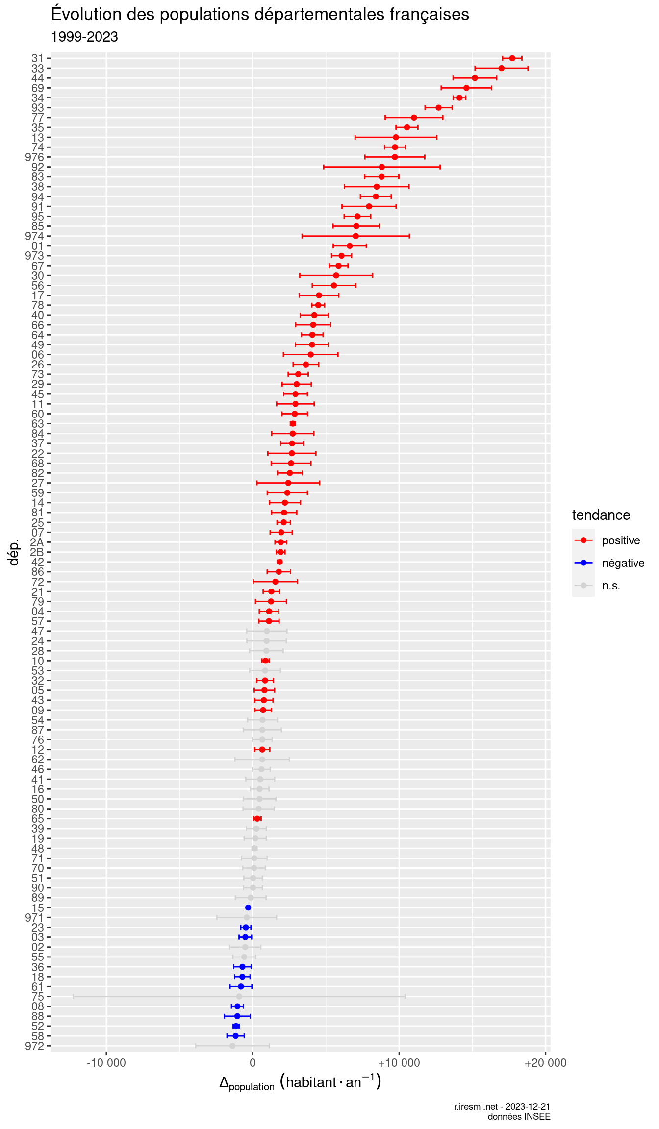

Only 10 départements have a clearly decreasing population

Map

pop_dep <- dep |> 
  inner_join(trends, join_by(insee_dep)) |>
  inner_join(filter(pop, 
                   annee == year_max, 
                   !insee_dep %in% c("F", "M")),
            join_by(insee_dep)) |> 
  st_transform("EPSG:2154") 

mean_fr <- trends |> 
  summarise(mean(estimate, na.rm = TRUE)) |> 
  pull()

world <- ne_countries(scale = "medium", returnclass = "sf") |> 
  filter(continent == "Europe") |> 
  st_transform("EPSG:2154") 

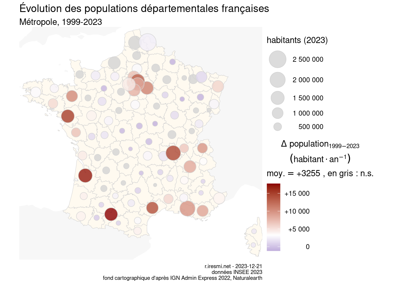
pop_dep |> 
  ggplot() +
  geom_sf(data = world, fill = "grey97", color = 0) +
  geom_sf(color = "lightgrey", fill = "floralwhite", size = .2) +
  stat_sf_coordinates(data = filter(pop_dep, p.value > .05),
                      aes(size = pop),
                      fill = "lightgrey", color = "lightgrey", shape = 21, alpha = 0.8) +
  stat_sf_coordinates(data = filter(pop_dep, p.value <= .05),
                      aes(size = pop, fill = estimate),
                      color = "lightgrey", shape = 21, alpha = 0.8) +
  coord_sf(xlim = c(160000, 1190000), 
           ylim = c(6085000, 7070000)) +
  scale_fill_gradient2(name = bquote(atop(displaystyle(atop(
                          Delta ~ population[.(year_min)-.(year_max)],
                          (habitant %.% an^{-1}))), 
                          moy. == .(sprintf("%+i", round(mean_fr))) ~ ", en gris : n.s.")),
                        labels = number_format(big.mark = " ", style_positive = "plus"),
                        low = "darkblue", mid = "white", high = "darkred", midpoint = mean_fr) +
  scale_size_area(name = glue("habitants ({year_max})"),
                  labels = number_format(big.mark = " "), 
                  max_size = 10) +
  guides(size = guide_legend(reverse = TRUE)) +
  labs(title = "Évolution des populations départementales françaises",
       subtitle = glue("Métropole, {year_min}-{year_max}"),
       x = "",
       y = "",
       caption = glue("r.iresmi.net - {Sys.Date()}
                      données INSEE {year_max}
                      fond cartographique d'après IGN Admin Express 2022, Naturalearth")) +
  theme_void() +
  theme(plot.caption = element_text(size = 7),
        legend.text.align = 1)

Figure 1: Population is growing stronger in Paris suburbs and in peripheral southern départements