library(raster)  # load before dplyr (against select conflict)
library(tidyverse)
library(httr)
library(sf)
library(btb)

# download and extract data
zipped_file <- tempfile()
GET("ftp://Admin_Express_ext:Dahnoh0eigheeFok@ftp3.ign.fr/ADMIN-EXPRESS_2-0__SHP__FRA_2019-03-14.7z.001",
    write_disk(zipped_file),
    progress())

system(paste("7z x -odata", zipped_file))

# create a unique polygon for France (our study zone)
fr <- read_sf("data/ADMIN-EXPRESS_2-0__SHP__FRA_2019-03-14/ADMIN-EXPRESS/1_DONNEES_LIVRAISON_2019-03-14/ADE_2-0_SHP_LAMB93_FR/REGION.shp") %>%
  st_union() %>%
  st_sf() %>%
  st_set_crs(2154)

# load communes ; convert to points
comm <- read_sf("data/ADMIN-EXPRESS_2-0__SHP__FRA_2019-03-14/ADMIN-EXPRESS/1_DONNEES_LIVRAISON_2019-03-14/ADE_2-0_SHP_LAMB93_FR/COMMUNE.shp")%>%
  st_set_crs(2154) %>%
  st_point_on_surface()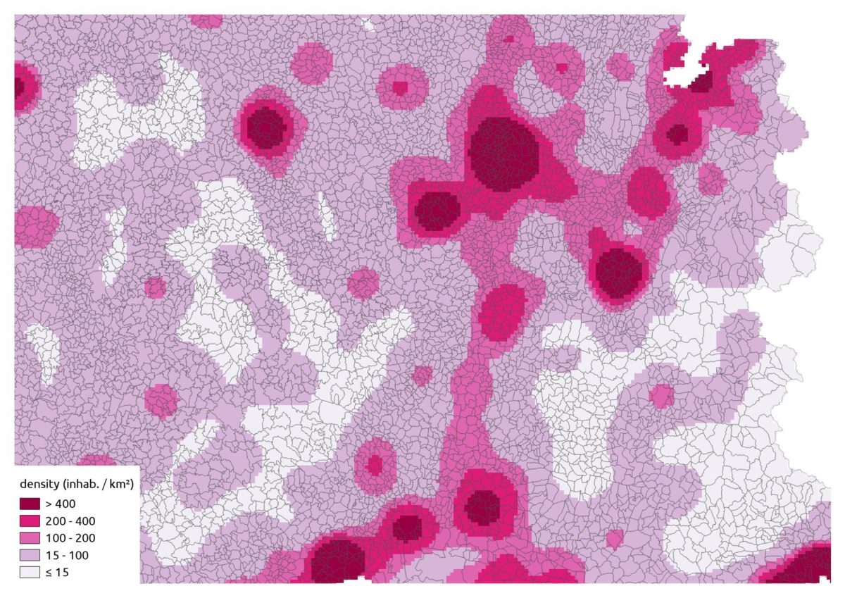
Representing mass data (inhabitants, livestock,…) on a map in not always easy : choropleth maps are clearly a no-go, except if you normalize with area and then you stumble on the MAUP… A nice solution is smoothing, producing a raster. You even get freebies like (potential) statistical confidentiality, a better geographic synthesis and easy multiple layers computations.
The kernel smoothing should not be confused with interpolation or kriging : the aim here is to « spread » and sum point values, see Loonis and de Bellefon (2018) for a comprehensive explanation.
We could use the {RSAGA} package which provides a « Kernel Density Estimation » in the « grid_gridding » lib for use with rsaga.geoprocessor(). However, we’ll use the {btb} package (Santos et al. 2018) which has the great advantage of providing a way to specify a geographical study zone, avoiding our values to bleed in another country or in the sea for example.
We’ll map the french population:
the data is available on the IGN site;
a 7z decompress utility must be available in your $PATH;
the shapefile COMMUNE.shp has a POPULATION field;
this is a polygon coverage, so we’ll take the « centroids ».
We create a function:
#' Kernel weighted smoothing with arbitrary bounding area
#'
#' @param df sf object (points)
#' @param field weight field in the df
#' @param bandwidth kernel bandwidth (map units)
#' @param resolution output grid resolution (map units)
#' @param zone sf study zone (polygon)
#' @param out_crs EPSG (should be an equal-area projection)
#'
#' @return a raster object
#' @import btb, raster, fasterize, dplyr, plyr, sf
lissage <- function(df, field, bandwidth, resolution, zone, out_crs = 3035) {
if (st_crs(zone)$epsg != out_crs) {
message("reprojecting data...")
zone <- st_transform(zone, out_crs)
}
if (st_crs(df)$epsg != out_crs) {
message("reprojecting study zone...")
df <- st_transform(df, out_crs)
}
zone_bbox <- st_bbox(zone)
# grid generation
message("generating reference grid...")
zone_xy <- zone %>%
dplyr::select(geometry) %>%
st_make_grid(cellsize = resolution,
offset = c(plyr::round_any(zone_bbox[1] - bandwidth, resolution, f = floor),
plyr::round_any(zone_bbox[2] - bandwidth, resolution, f = floor)),
what = "centers") %>%
st_sf() %>%
st_join(zone, join = st_intersects, left = FALSE) %>%
st_coordinates() %>%
as_tibble() %>%
dplyr::select(x = X, y = Y)
# kernel
message("computing kernel...")
kernel <- df %>%
cbind(., st_coordinates(.)) %>%
st_set_geometry(NULL) %>%
dplyr::select(x = X, y = Y, field) %>%
btb::kernelSmoothing(dfObservations = .,
sEPSG = out_crs,
iCellSize = resolution,
iBandwidth = bandwidth,
vQuantiles = NULL,
dfCentroids = zone_xy)
# rasterization
message("\nrasterizing...")
raster::raster(xmn = plyr::round_any(zone_bbox[1] - bandwidth, resolution, f = floor),
ymn = plyr::round_any(zone_bbox[2] - bandwidth, resolution, f = floor),
xmx = plyr::round_any(zone_bbox[3] + bandwidth, resolution, f = ceiling),
ymx = plyr::round_any(zone_bbox[4] + bandwidth, resolution, f = ceiling),
resolution = resolution) %>%
fasterize::fasterize(kernel, ., field = field)
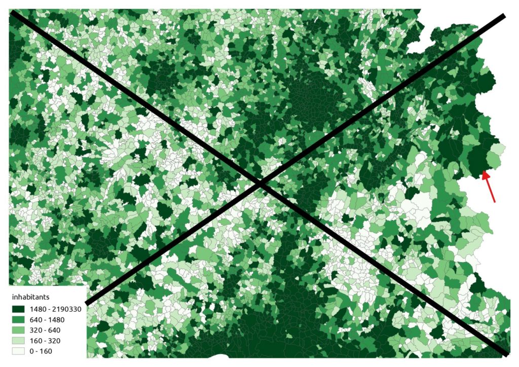
}Instead of a raw choropleth map like this (don’t do this at home):
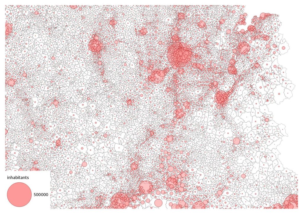
… we should use a proportional symbol. But it’s quite cluttered in urban areas:
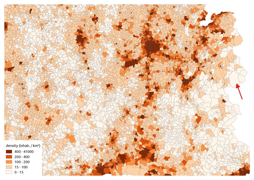
We can also get the polygon density:
We just have to run our function for example with a bandwidth of 20 km and a cell size of 2 km. We use an equal area projection: the LAEA Europa (EPSG:3035).
comm %>%
  lissage("POPULATION", 20000, 2000, fr, 3035) %>%
  raster::writeRaster("pop.tif")
And lastly our smoothing:
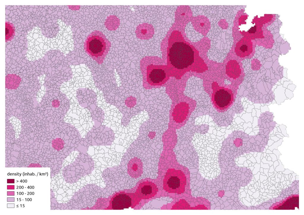
That’s a nice synthetic representation!
After that it’s easy in R to do raster algebra; for example dividing a grid of crop yields by a grid of agricultural area, create a percent change between dates, etc.
As a conclusion, a quote:
Behind the aesthetic quality of the smoothed maps, however, lies a major trap. By construction, smoothing methods mitigate breakdowns and borders and induce continuous representation of geographical phenomena. The smoothed maps therefore show the spatial autocorrelation locally.Two points close to the smoothing radius have mechanically comparable characteristics in this type of analysis. As a result, there is little point in drawing conclusions from a smoothed map of geographical phenomena whose spatial scale is of the order of the smoothing radius.
Loonis and de Bellefon (2018)
References
Loonis, Vincent, and Marie-Pierre de Bellefon, eds. 2018. Handbook of Spatial Analysis. Theory and Application with R. INSEE Méthodes 131. Institut national de la statistique et des études économiques. https://www.insee.fr/en/information/3635545.
Santos, Arlindo Dos, Francois Semecurbe, Auriane Renaud, Cynthia Faivre, Thierry Cornely, and Farida Marouchi. 2018. Btb: Beyond the Border - Kernel Density Estimation for Urban Geography. https://CRAN.R-project.org/package=btb.