remotes::install_gitlab("mdagr/itra")
library(itra)
library(tidyverse)
library(glue)
library(hms)
library(lubridate)
library(gghighlight)
library(progress)
Trail running can be hard (Malliaropoulos et al. 2015; Hespanhol Junior et al. 2017; Istvan et al. 2019; Messier et al. 2018). During one, I was wondering if we can avoid the race completely and predict the race time according to distance, elevation change, sex and performance index (so yes, we have to run sometimes to measure it first).
We need a dataset to play with. ITRA maintains a quite comprehensive database (International Trail Running Association 2020), but no current dataset is openly available. However we can use the hidden JSON API to scrape a sample. I created a R package {itra} for this purpose ; with it we can get some runners and their results:
NOTE (2021-09): the ITRA website has changed, so the package doesn’t work any longer.
A test:
itra_runners("jornet")# A tibble: 5 x 15
id_coureur id cote nom prenom quartz team M L XL XXL
<int> <int> <int> <chr> <chr> <int> <chr> <int> <lgl> <lgl> <int>
1 2704 2.70e3 950 JORN… Kilian 20 "" 898 NA NA 896
2 707322 7.07e5 538 RENU… Arturo 0 "" NA NA NA NA
3 2667939 2.67e6 520 PARE… Samuel 0 "" NA NA NA NA
4 2673933 2.67e6 468 PÉRE… Anna 0 "" NA NA NA NA
5 2673935 2.67e6 468 RIUS… Sergi 0 "" NA NA NA NA
# … with 4 more variables: S <int>, XS <int>, XXS <lgl>, palmares <chr>It works worked…
Get the data
So, we’re going to build a dataframe of single letters and random page index to create our dataset of runners. I’ll manually add some low index to oversample the elite athletes otherwise we will probably miss them entirely.
# helpers -----------------------------------------------------------------

# compute the mode (to find the runner sex from its details ; see below)
stat_mode <- function(x, na.rm = FALSE) {
  if(na.rm) {
    x <- x[!is.na(x)]
  }

  ux <- unique(x)
  ux[which.max(tabulate(match(x, ux)))]
}


# sample -------------------------------------------------------------

# progress bar versions of ITRA functions (scraping will be slow, we want to know if it works)
pb_itra_runners <- function(...) {
  pb$tick()
  itra_runners(...)
}

pb_itra_runner_results <- function(...) {
  pb$tick()
  itra_runner_results(...)
}

pb_itra_runner_details <- function(...) {
  pb$tick()
  itra_runner_details(...)
}

# dataset generation from a "random" set of index
#
oversample_high_score <- c(0, 50, 100, 250, 500)
my_sample <- tibble(l = letters,
                 n = c(oversample_high_score,
                       sample(0:100000,
                              length(letters) - length(oversample_high_score)))) |>
  expand(l, n) |>
  distinct(l, n)
We have 676 tuples of (letter, index). We can now start querying the website, we should get 5 runners (by default) for each tuple. But we will have some duplicates because for example at index 0 we will get « Kilian Jornet » for the letters « k », « i », « l »…
I use purr::map2 to iterate along our sample, using slowly to avoid overloading the website and possibly to get NA instead of stopping errors.
You’ll see that the JSON variables have french or english names!
#  querying runners --------

pb <- progress_bar$new(format = "[:bar] :current/:total remaining: :eta",
             total = nrow(my_sample))

my_dataset <- my_sample |>
  mutate(runners = map2(l, n, possibly(slowly(pb_itra_runners, rate_delay(.5)), NA)))

# runners list
runners <- my_dataset |>
  drop_na(runners) |>
  unnest(runners) |>
  distinct(id_coureur, .keep_all = TRUE) |>
  select(-l, -n)
Here instead of the nominal 3380 runners I get only 2796…
Then we can query for their race results and their sex.
pb <- progress_bar$new(format = "[:bar] :current/:total remaining: :eta",
                       total = nrow(runners))
results <- runners |>
  select(id, first_name = prenom, last_name = nom) |>
  mutate(runner_results = pmap(., possibly(slowly(pb_itra_runner_results, rate_delay(.5)), NA))) |>
  unnest(runner_results)

# performance index by trail category and sex
pb <- progress_bar$new(format = "[:bar] :current/:total remaining: :eta",
             total = nrow(runners))
runners_details <- runners |>
  select(id) |>
  mutate(details = map(id, possibly(slowly(pb_itra_runner_details, rate_delay(.5)), NA))) |>
  unnest(details)
Some preprocessing is necessary. Sex is not a direct property of the runners, we must get it from runners_details. We then join our 3 dataframes and compute some new variables.
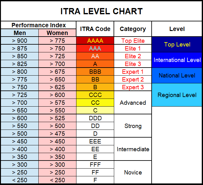
Levels come from:
# preprocessing ----
runners_sex <- runners_details |>
  group_by(id) |>
  summarise(sex = stat_mode(sexe, na.rm = TRUE))

results_clean <- results |>
  rename(cote_course = cote) |>
  left_join(select(runners, -nom, -prenom), by = "id") |>
  left_join(runners_sex, by = "id") |>
  mutate(dist_tot = as.numeric(dist_tot),
       dt = ymd(dt),
       time = lubridate::hms(temps),
       hours = as.numeric(time, "hours"),
       kme = dist_tot + deniv_tot / 100,
       level = factor(
                  case_when(
                   (cote > 825 & sex == "H") | (cote > 700 & sex == "F") ~ "elite",
                   (cote > 750 & sex == "H") | (cote > 625 & sex == "F") ~ "expert",
                   (cote > 650 & sex == "H") | (cote > 550 & sex == "F") ~ "advanced",
                   (cote > 500 & sex == "H") | (cote > 475 & sex == "F") ~ "strong",
                   (cote > 350 & sex == "H") | (cote > 350 & sex == "F") ~ "intermediate",
                   is.na(sex) ~ NA_character_,
                   TRUE ~ "novice"),
                 levels = c("novice", "intermediate", "strong", "advanced", "expert", "elite")))
Exploratory analysis
Having a quick look at the dataset…
# analysis -----------------------------------------------------------------

# runners' ITRA performance index
runners |>
  left_join(runners_sex) |>
  ggplot(aes(cote, fill = sex)) +
    geom_histogram(binwidth = 10)
# distance ran
results_clean |>
  ggplot(aes(dist_tot)) +
    geom_histogram(binwidth = 2)
# times ran
results_clean |>
  ggplot(aes(hours)) +
    geom_histogram(binwidth = 1 / 6)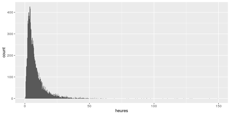
# by level
results_clean |>
  drop_na(level) |>
  filter(hours != 0) |>
  ggplot(aes(kme, hours, color = level)) +
    geom_point(alpha = .3) +
    gghighlight() +
    coord_cartesian(xlim = c(0, 320), ylim = c(0, 65)) +
    facet_wrap(~ level)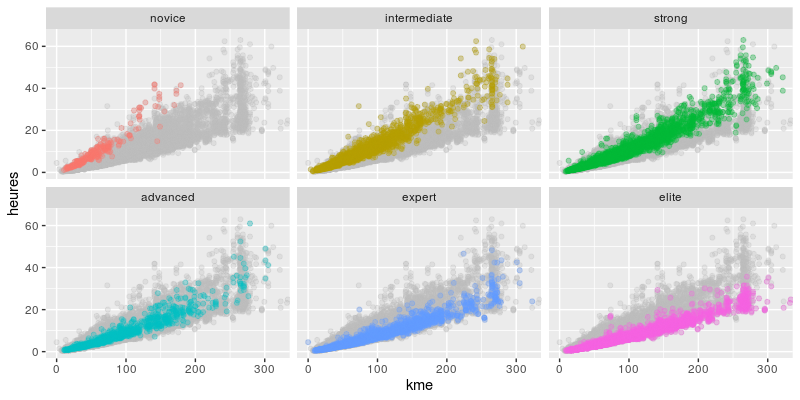
Prediction
Now, back to my initial question. Can I just predict my race time and avoid a long pain by not running?
I will use a random forest. Since the rows are not independent (we have several results per runner), I use a group kfold on the runner id.
library(caret)
library(ranger)

results_rf <- results_clean |>
  drop_na(hours, cote)

# grouped CV folds
group_fit_control <- trainControl(
  index = groupKFold(results_rf$id, k = 10),
  method = "cv")

rf_fit <- train(hours ~ dist_tot + deniv_tot + deniv_neg_tot + cote + sex,
        data = results_rf,
        method = "rf",
        trControl = group_fit_control)
rf_fit
Random Forest
18339 samples
5 predictors
No pre-processing
Resampling: Cross-Validated (10 fold)
Summary of sample sizes: 16649, 16704, 16338, 16524, 16407, 16223, ...
Resampling results across tuning parameters:
mtry splitrule RMSE Rsquared MAE
2 variance 1.822388 0.9472348 0.8747978
2 extratrees 1.844228 0.9463288 0.8810525
3 variance 1.827556 0.9469227 0.8801065
3 extratrees 1.847274 0.9459055 0.8800262
5 variance 1.873645 0.9440697 0.9021319
5 extratrees 1.853316 0.9455854 0.8882530
Tuning parameter 'min.node.size' was held constant at a value of 5
RMSE was used to select the optimal model using the smallest value.
The final values used for the model were mtry = 2, splitrule = variance
and min.node.size = 5.So with a root mean square error of 1.82 hours, I can’t say that my model is super precise. However in my case, my last 16 km (01:40:00) is pretty well predicted!
predict(rf_fit, newdata = tibble(dist_tot = 16,
                 deniv_tot = 600,
                 deniv_neg_tot = 600,
                 cote = 518,
                 sex = "H")) |>
  magrittr::multiply_by(3600) |>
  floor() |>
  seconds_to_period() |>
  hms::hms()
# 01:37:42
So next time I’ll just run the model instead of running the race.
I’ll leave the tuning to the specialists. While writing this post I found another (Fogliato et al. 2020) potential similar use for the {itra} package.
References
Fogliato, Riccardo, Natalia L. Oliveira, and Ronald Yurko. 2020. “TRAP: A Predictive Framework for Trail Running Assessment of Performance.” arXiv:2002.01328 [Stat], ahead of print, July. https://doi.org/10.48550/ARXIV.2002.01328.
Hespanhol Junior, Luiz Carlos, Willem Van Mechelen, and Evert Verhagen. 2017. “Health and Economic Burden of Running-Related Injuries in Dutch Trailrunners: A Prospective Cohort Study.” Sports Medicine 47 (2): 367–77. https://doi.org/10.1007/s40279-016-0551-8.
International Trail Running Association. 2020. “ITRA.” In International Trail Running Association. https://itra.run/.
Istvan, Albertus Oosthuizen, Paul Yvonne, Jeremy Ellapen Terry, et al. 2019. “Common Ultramarathon Trail Running Injuries and Illnesses: A Review (2007-2016).” International Journal of Medicine and Medical Sciences 11 (4): 36–42. https://doi.org/10.5897/IJMMS2018.1386.
Malliaropoulos, Nikolaos, Dimitra Mertyri, and Panagiotis Tsaklis. 2015. “Prevalence of Injury in Ultra Trail Running.” Human Movement 16 (2). https://doi.org/10.1515/humo-2015-0026.
Messier, Stephen P., David F. Martin, Shannon L. Mihalko, et al. 2018. “A 2-Year Prospective Cohort Study of Overuse Running Injuries: The Runners and Injury Longitudinal Study (Trails).” The American Journal of Sports Medicine 46 (9): 2211–21. https://doi.org/10.1177/0363546518773755.