---
title: "Population growth"
description: "Cats, many cats"
author: "Michaël"
date: "2023-02-10"
date-modified: last-modified
categories:
- R
- ecology
draft: false
freeze: true
editor_options:
chunk_output_type: console
---
[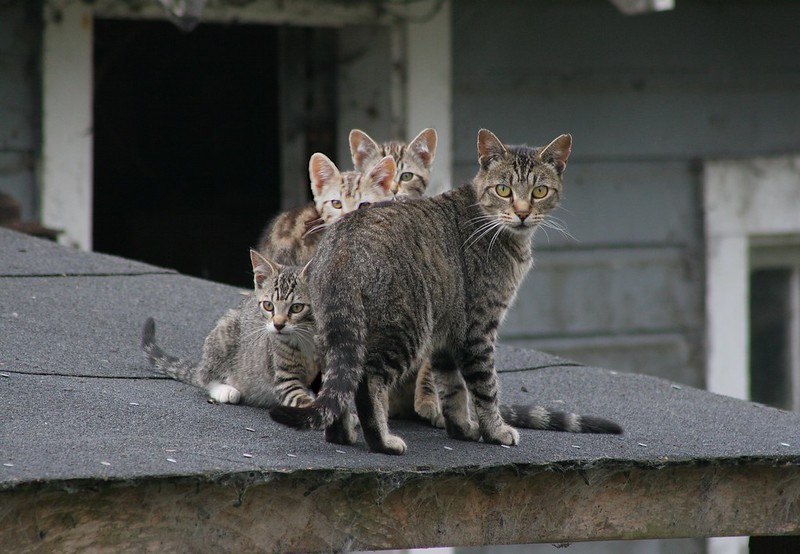{fig-alt="A photo of a feral Cat Mom and 3 Kittens"}](https://flic.kr/p/71QYq8)
I just saw [this article](https://www.lemonde.fr/m-perso/article/2023/02/09/le-chat-ce-fleau-ecologique_6161170_4497916.html) in *Le Monde*:
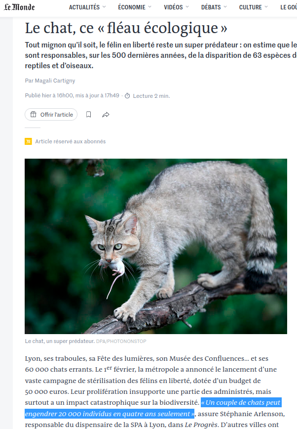{fig-alt="Newspaper screenshot: A pair of cats can produce 20,000 individuals in just four years"}
> « a pair of cats can produce 20,000 individuals in just four years ».
>
> *(translation)*
That seems quite high... Let's check!
::: callout-note
Additionally, the article is about [feral cats](https://en.wikipedia.org/wiki/Feral_cat) preying on wildlife but we are shown a picture of a [wild cat](https://en.wikipedia.org/wiki/European_wildcat) capturing a laboratory mouse!
:::
This figure could come from a back-of-the-envelope calculation, such as litters of 3.5 kitten twice a year for 4 years producing 3.5^8^ ≈ 22,519 kitten. But that's a very rough and false estimate: at this rate there will be 76 billions cats in Lyon in 10 years! Moreover we ignore the fact that the first generations can still have litters, the less than perfect survival of feral cats, the delay before the first pregnancy, *etc.*
We can use [Leslie matrix](https://en.wikipedia.org/wiki/Leslie_matrix) to model the destiny of our founding pair. Leslie matrices are used in population ecology to project a structured (by age) population based on transitions between age classes and fertility.
Cat females reach sexual maturity at 6--8 months [@KaeufferEffectivesizetwo2004], can have 2.1 litters each year [@RobinsonReproductiveperformancecat1970] and have a mean of around 4 kitten by litter [@HallLittersizebirth1934; @Deagconsequencesdifferenceslitter1987] or 9.1 kitten by year [@RobinsonReproductiveperformancecat1970]. So we will use quarters as ages classes. We first use an unrealistic 100 % survival and 100 % fecundity.
## R base version
The first line of the matrix reads 0 kitten produced between 0-3 months, 0 kitten between 3-6 months, and $9.1 / 2 / 4 = 1.4$ kitten by capita by quarter for the 6-9 months class and the adults. The 1s on the diagonal are the survivals between age classes and the lower-right 1 the adult survival.
```{r}
l <- matrix(c(0, 0, 1.4, 1.4,
              1, 0,   0,   0,
              0, 1,   0,   0,
              0, 0,   1,   1),
            nrow = 4,
            byrow = TRUE)

quarters <- 16

n0 <- matrix(c(0, 0, 0, 2),
             ncol = 1)

simul <- function(q) {
  n_proj <- matrix(0,
                   nrow = nrow(l),
                   ncol = q)
  n_proj[, 1] <- n0

  for (i in 1:(q - 1)) {
    n_proj[, i + 1] <- l %*% n_proj[, i]
  }
  return(n_proj)
}

res <- simul(quarters)
(final_pop <- round(sum(res[, ncol(res)])))
```
**With our optimistic parameters, we get a population of around `r round(final_pop, -1)` cats after `r quarters` quarters (`r quarters / 4` years). An order of magnitude less than in the article...**
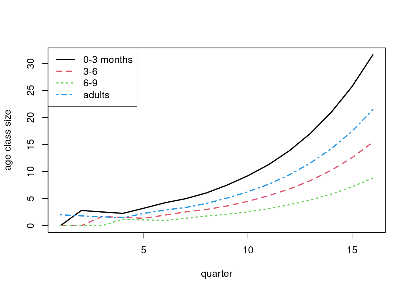
With a more realistic matrix, especially for feral cats, with less fertility for the first pregnancy and survival rates totally made-up but not 100 %, we can get quite a more manageable population size:
```{r}
l <- matrix(c(0,     0,   1, 1.4,
              0.6,   0,   0,   0,
              0,   0.7,   0,   0,
              0,     0, 0.8,  .9),
            nrow = 4,
            byrow = TRUE)

res <- simul(quarters)
(final_pop_2 <- round(sum(res[, ncol(res)])))
round(res)
matplot(1:quarters, t(res), type = "l", lty = 1:ncol(l),
        xlab = "quarter", ylab = "age class size", lwd = 2)
legend("topleft", legend = c("0-3 months", "3-6", "6-9", "adults"),
       lty = 1:ncol(l), col = 1:ncol(l), lwd = 2)
```
So only `r final_pop_2` cats now... I let you play with fertility and survival rates to stabilize the population.
But anyway, cats do have an effect on wildlife, so whatever their population size, we must act to reduce their impact.
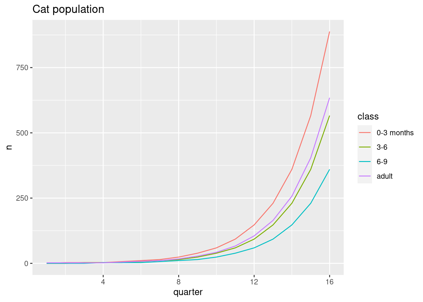
## Tidyverse version
```{r}
library(tidyverse)

l <- matrix(c(0, 0, 1.4, 1.4,
              1, 0,   0,   0,
              0, 1,   0,   0,
              0, 0,   1,   1),
            nrow = 4,
            byrow = TRUE)

quarters <- 16

n0 <- matrix(c(0, 0, 0, 2),
             ncol = 1)

res <- list(l) |>
  rep(quarters - 1) |>
  accumulate(`%*%`, .init = n0, .dir = "backward") |>
  rev() |>
  bind_cols(.name_repair = "unique_quiet")

res |>
  summarise(across(last_col(), sum))
res |>
  mutate(class = c("0-3 months", "3-6", "6-9", "adult"), .before = 1) |>
  pivot_longer(-1,
               names_to = "quarter",
               values_to = "n",
               names_prefix = "...",
               names_transform = as.integer) |>
  ggplot(aes(quarter, n)) +
  geom_line(aes(color = class)) +
  labs(title = "Cat population")
```
## References
::: {#refs}
:::