---
title: "Cherry blossom"
description: "Plant physiology and climate"
author: "Michaël"
date: "2023-04-05T18:00:00"
date-modified: last-modified
categories:
- R
- datavisualization
draft: false
freeze: true
editor_options:
chunk_output_type: console
---
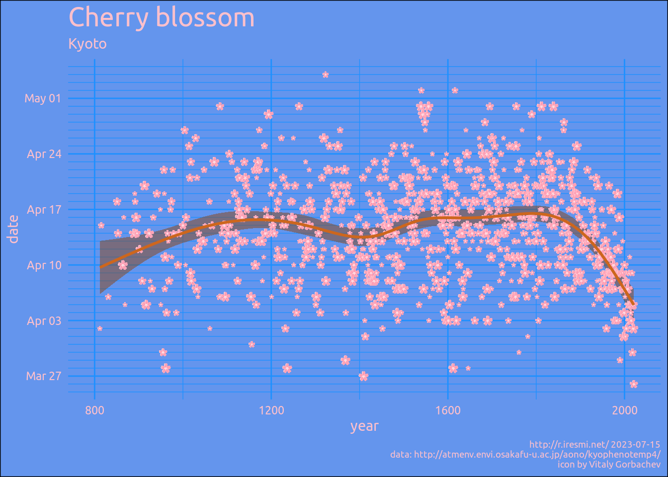
It's cherry blossom time...
A nice dataset going back to the year 812 in Japan can be found [here](http://atmenv.envi.osakafu-u.ac.jp/aono/kyophenotemp4/). It describes the phenological data for full flowering date of cherry tree (*Prunus jamasakura*) in Kyoto, showing springtime climate changes.
[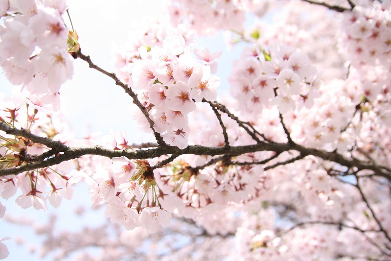](https://flic.kr/p/bBA3Hu)
Let's draw...
```{r}
# params ------------------------------------------------------------------

url_kyoto <- "http://atmenv.envi.osakafu-u.ac.jp/aono/kyophenotemp4/"
file_kyoto <- "kyoto.rds"   # cache data
icon_sakura <- "sakura.png" # cache icon


# config ------------------------------------------------------------------

library(tidyverse)
library(fs)
library(janitor)
library(httr)
library(rvest)
library(glue)
library(ggimage)

invisible(Sys.setlocale("LC_TIME", "en_GB.UTF-8"))


# data --------------------------------------------------------------------

# icon
if (!file_exists(icon_sakura)) {
  GET("https://www.flaticon.com/download/icon/7096433?icon_id=7096433&author=232&team=232&keyword=Sakura&pack=packs%2Fsakura-festival-59&style=522&format=png&color=&colored=2&size=512&selection=1&premium=0&type=standard&search=cherry+blossom",
      write_disk(icon_sakura))
}

# blossom dates, scraped from the web page (more up to date than the xls files)
if (!file_exists(file_kyoto)) {
  GET(url_kyoto) |>
    content() |>
    html_element("pre") |>
    html_text2() |>
    str_replace_all("\xc2\xa0", " ") |> # bad encoding needs correction
    read_fwf(fwf_cols("ad"   = c(7, 10),
                      "fifd" = c(17, 20),
                      "fufd" = c(22, 25),
                      "work" = c(27, 30),
                      "type" = c(32, 35),
                      "ref"  = c(37, Inf)),
             skip = 26,
             na = c("", "NA", "-")) |>
    remove_empty() |>
    mutate(full_flowering_date = ymd(glue("{str_pad(ad, 4, 'left', '0')}{fufd}")),
           full_flowering_date_doy = yday(full_flowering_date)) |>
    write_rds(file_kyoto)
}


# plot --------------------------------------------------------------------

read_rds(file_kyoto) |>
  mutate(random_size = sample(c(0.015, 0.02, 0.025, 0.03), length(ad), replace = TRUE)) |>
  ggplot(aes(ad, parse_date_time(full_flowering_date_doy, orders = "j"))) +
  geom_smooth(color = NA, fill = "chocolate4", alpha = 0.5) +
  geom_image(aes(size = I(random_size)), image = icon_sakura) +
  geom_smooth(color = "chocolate3", se = FALSE, alpha = 0.5) +
  scale_y_datetime(labels = scales::date_format("%b %d"),
                   breaks = "weeks", minor_breaks = "days") +
  labs(title = "Cherry blossom",
       subtitle = "Kyoto",
       x = "year",
       y = "date",
       caption = glue("http://r.iresmi.net/ {Sys.Date()}
                      data: {url_kyoto}
                      icon by Vitaly Gorbachev")) +
  theme_minimal() +
  theme(plot.background = element_rect(fill = "cornflowerblue"),
        panel.grid = element_line(color = "dodgerblue"),
        text = element_text(color = "pink", family = "Ubuntu"),
        plot.title = element_text(size = 20),
        plot.caption = element_text(size = 7),
        axis.text = element_text(color = "pink"))
ggsave("cherry_blossom.png", width = 25, height = 18, units = "cm", dpi = 300)
```