---
title: "Where and when (not) to eat in France?"
description: "To eat or not to eat..."
author: "Michaël"
date: "2023-04-16"
date-modified: last-modified
categories:
- R
- datavisualization
- spatial
draft: false
freeze: true
code-fold: true
code-tools: true
editor_options:
chunk_output_type: console
---
Results of sanitary controls in France can be found on [data.gouv.fr](https://www.data.gouv.fr/fr/datasets/resultats-des-controles-officiels-sanitaires-dispositif-dinformation-alimconfiance/) however, only the running year is available... Thanks to [\@cquest\@amicale.net](https://amicale.net/@cquest) we can access the [archives](https://www.opendatarchives.fr/) since 2017.
## Config and data cleaning
```{r}
#| label: config
library(tidyverse)
library(janitor)
library(fs)
library(sf)
library(glue)
library(ggspatial)
library(rnaturalearth)
library(patchwork)

# smoothing
source(glue("fonctions_lissage.R"), encoding = "UTF-8")

# move DROM
source(glue("translation.R"), encoding = "UTF-8")

# params ------------------------------------------------------------------

rayon <- 30000 # smoothing radius (m)
pixel <- 2000  # pixel resolution output for smoothing (m)
proj_liss <- "EPSG:3035" # an equal area projection
```
```{r}
#| label: data
# 2017-2018 : yearly archive ; extract the last doy export
#
# http://data.cquest.org/alim_confiance/exports_alim_confiance_2017.7z
#  -> export_alimconfiance_2017-12-31.csv
# http://data.cquest.org/alim_confiance/exports_alim_confiance_2018.7z
#  -> export_alimconfiance_2018-12-31.csv
alim_dcq <- dir_ls("data/data.cquest.org", regexp = "\\.csv") |>
  map_dfr(read_csv2) |>
  clean_names()

# 2019-2023
# archives at the end of each year + last export
#
# http://files.opendatarchives.fr/dgal.opendatasoft.com/archives/export_alimconfiance/20191231T053939Z%20export_alimconfiance.csv.gz
# http://files.opendatarchives.fr/dgal.opendatasoft.com/archives/export_alimconfiance/20201231T083455Z%20export_alimconfiance.csv.gz
# http://files.opendatarchives.fr/dgal.opendatasoft.com/archives/export_alimconfiance/20211231T083316Z%20export_alimconfiance.csv.gz
# http://files.opendatarchives.fr/dgal.opendatasoft.com/archives/export_alimconfiance/20221231T150844Z%20export_alimconfiance.csv.gz
# http://files.opendatarchives.fr/dgal.opendatasoft.com/export_alimconfiance.csv.gz
alim_oda <- dir_ls("data/files.opendatarchives.fr", regexp = "\\.csv") |>
  map_dfr(read_csv2) |>
  clean_names() |>
  distinct() |>
  filter(date_inspection < "2023-03-01")

# https://datanova.laposte.fr/explore/dataset/laposte_hexasmal/download?format=shp
cp <- read_sf("~/data/laposte/laposte_hexasmal.shp")

# Built from IGN Adminexpress. Get the data :
# https://r.iresmi.net/posts/2021/simplifying_polygons_layers/results/adminexpress_simpl_2022.zip
dep <- read_sf("~/data/adminexpress/adminexpress_cog_simpl_000_2022.gpkg",
               layer = "departement") |>
  translater_drom(ajout_zoom_pc = TRUE)

reg_fx <- read_sf("~/data/adminexpress/adminexpress_cog_simpl_000_2022.gpkg",
               layer = "region") |>
  filter(insee_reg > "06")

fx <- read_sf("~/data/adminexpress/adminexpress_cog_simpl_000_2022.gpkg",
              layer = "region") |>
  filter(insee_reg > "06") |>
  summarise() |>
  st_transform(proj_liss)

# projection names
nom_proj_liss <- str_extract(st_crs(fx)$wkt, '(?<=PROJCRS\\[").*(?=",)')
nom_proj_legale <- str_extract(st_crs(dep)$wkt, '(?<=PROJCRS\\[").*(?=",)')

# basemap
countries <- ne_countries(50, returnclass = "sf") |>
  filter(admin != "France")
```
```{r}
#| label: preprocessing
alim_raw <- bind_rows(alim_dcq,
                      alim_oda) |>
  mutate(insee_dep = case_when(str_sub(code_postal, 1, 2) >= "97" ~ str_sub(code_postal, 1, 3),
                         str_sub(code_postal, 1, 3) %in% c("200", "201") ~ "2A",
                         str_sub(code_postal, 1, 3) %in% c("202", "206") ~ "2B",
                         TRUE ~ str_sub(code_postal, 1, 2)))


# trying to add coordinates to unknown locations using postal codes
# only 5800 on 7500
georef <- cp |>
  group_by(code_postal) |>
  summarise(geometry = first(geometry)) |>
  inner_join(alim_raw |>
              filter(is.na(geores),
                     !is.na(code_postal)),
             by = "code_postal")

# build sf object
alim <- alim_raw |>
  filter(!is.na(geores)) |>
  separate(geores, c("y", "x"), sep = ",") |>
  st_as_sf(coords = c("x", "y"), crs = "EPSG:4326") |>
  bind_rows(georef)

alim |>
  write_sf(glue("results/alim.gpkg"))
```
## Exploring data
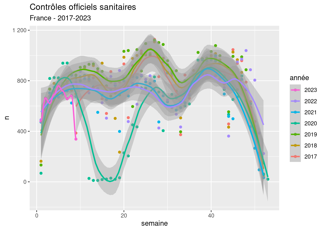
First a global view of the dataset:
```{r}
#| label: fig-week
#| fig-cap: Overview by week
#| fig-alt: A scatter plot with smoothed lines showing the number of controls by week and year
alim |>
  st_drop_geometry() |>
  count(annee = year(date_inspection),
        semaine = isoweek(date_inspection)) |>
  ggplot(aes(semaine, n, group = annee, color = as_factor(annee))) +
  geom_point() +
  geom_smooth(span = 0.4) +
  scale_y_continuous(labels = scales::label_number(big.mark = " ")) +
  labs(title = "Contrôles officiels sanitaires",
       subtitle = "France - 2017-2023",
       color = "année") +
  guides(color = guide_legend(reverse=TRUE))
```
About 800 controls per week, except during the lock-down in 2020, and a slightly lower control pressure in 2021 and 2022.
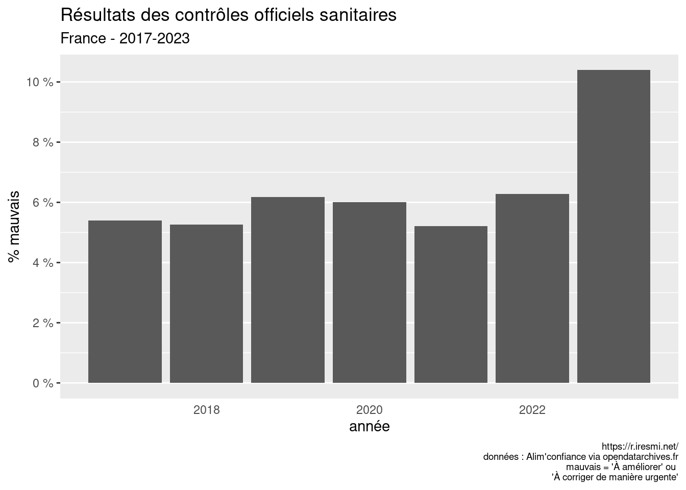
```{r}
#| label: fig-year
#| fig-cap: Yearly
#| fig-alt: A bar plot of bad controls by year
alim |>
  st_drop_geometry() |>
  group_by(annee = year(date_inspection)) |>
  summarise(pcent_neg = sum(synthese_eval_sanit %in% c("A améliorer", "A corriger de manière urgente")) / n()) |>
  ggplot(aes(annee, pcent_neg)) +
  geom_col() +
  scale_y_continuous(breaks = scales::breaks_pretty(),
                     labels = scales::label_percent(decimal.mark = ",", suffix = " %")) +
  labs(title = "Résultats des contrôles officiels sanitaires",
       subtitle = "France - 2017-2023",
       x = "année",
       y = "% mauvais",
       caption = glue("https://r.iresmi.net/
                     données : Alim'confiance via opendatarchives.fr
                     mauvais = 'À améliorer' ou
                       'À corriger de manière urgente'")) +
  theme(panel.grid.major.x = element_blank(),
        panel.grid.minor.x = element_blank(),
        axis.ticks.x = element_blank(),
        plot.caption = element_text(size = 7))
```
Poor results (*To be improved* or *To be corrected urgently*) are stable at around 6 %, except a recent spike in 2023?
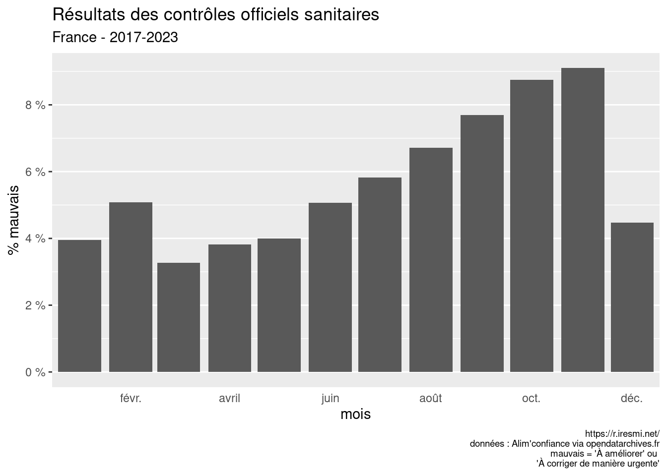
```{r}
#| label: fig-month
#| fig-cap: Monthly
#| fig-alt: A bar plot of bad controls by month
alim |>
  st_drop_geometry() |>
  group_by(mois = ymd(paste0("2020", str_pad(month(date_inspection), 2, "left", "0"), "01"))) |>
  summarise(pcent_neg = sum(synthese_eval_sanit %in% c("A améliorer", "A corriger de manière urgente")) / n()) |>
  ggplot(aes(mois, pcent_neg)) +
  geom_col() +
  scale_x_date(date_labels = "%b", date_breaks = "2 months", expand = c(0.01, 0.01)) +
  scale_y_continuous(breaks = scales::breaks_pretty(),
                     labels = scales::percent_format(decimal.mark = ",", suffix = " %")) +
  labs(title = "Résultats des contrôles officiels sanitaires",
       subtitle = "France - 2017-2023",
       y = "% mauvais",
       caption = glue("https://r.iresmi.net/
                     données : Alim'confiance via opendatarchives.fr
                     mauvais = 'À améliorer' ou
                       'À corriger de manière urgente'")) +
  theme(panel.grid.major.x = element_blank(),
        panel.grid.minor.x = element_blank(),
        axis.ticks.x = element_blank(),
        plot.caption = element_text(size = 7))
```
It seems that poor results increase during the year, from June to November.
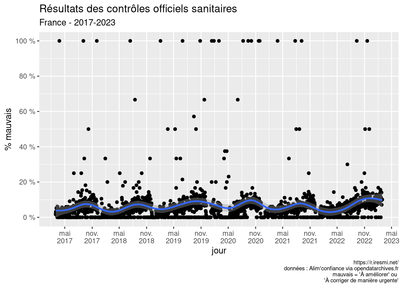
This surprising periodic phenomenon is also visible by day:
```{r}
#| label: fig-day
#| fig-cap: Daily
#| fig-alt: A bar plot of bad controls by day with a smooth line
alim |>
  st_drop_geometry() |>
  group_by(date_inspection = as.Date(date_inspection)) |>
  summarise(pcent_neg = sum(synthese_eval_sanit %in% c("A améliorer", "A corriger de manière urgente")) / n()) |>
  ggplot(aes(date_inspection, pcent_neg)) +
  geom_point() +
  geom_smooth(method = "gam", formula = y ~ s(x, bs = "cs", k = 30)) +
  scale_x_date(labels = ~ format(.x, "%b\n%Y"), date_breaks = "6 months") +
  scale_y_continuous(breaks = scales::breaks_pretty(),
                     labels = scales::percent_format(decimal.mark = ",", suffix = " %")) +
  labs(title = "Résultats des contrôles officiels sanitaires",
       subtitle = "France - 2017-2023",
       x = "jour",
       y = "% mauvais",
       caption = glue("https://r.iresmi.net/
                     données : Alim'confiance via opendatarchives.fr
                     mauvais = 'À améliorer' ou
                       'À corriger de manière urgente'")) +
  theme(plot.caption = element_text(size = 7))
```
So for the « when », it is: not in summer or autumn.
## Maps
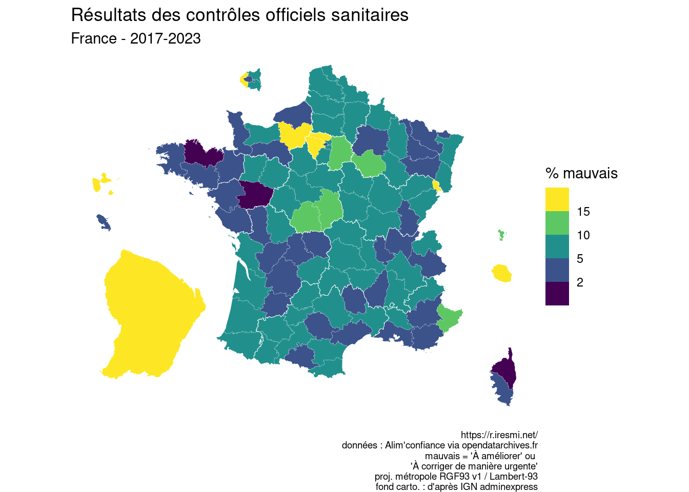
What about the « where »? It seems you also could be careful in some départements...
```{r}
#| label: fig-full-dep
#| fig-cap: All controls (by dép.)
#| fig-alt: A map of bad controls by département of France
bilan_dep <- alim |>
  st_drop_geometry() |>
  group_by(insee_dep) |>
  summarise(pcent_neg = sum(synthese_eval_sanit %in% c("A améliorer", "A corriger de manière urgente")) / n() * 100) |>
  arrange(desc(pcent_neg))

dep |>
  left_join(bilan_dep, by = "insee_dep") |>
  ggplot() +
  geom_sf(aes(fill = pcent_neg), color = "white", linewidth = 0.05) +
  geom_sf(data = reg_fx, fill = NA, color = "white", linewidth = .1) +
  scale_fill_viridis_b("% mauvais", breaks = c(2, 5, 10, 15), na.value = NA) +
  labs(title = "Résultats des contrôles officiels sanitaires",
       subtitle = "France - 2017-2023",
       caption = glue("https://r.iresmi.net/
                     données : Alim'confiance via opendatarchives.fr
                     mauvais = 'À améliorer' ou
                       'À corriger de manière urgente'
                     proj. métropole {nom_proj_legale}
                     fond carto. : d'après IGN adminexpress")) +
  theme_void() +
  theme(plot.caption = element_text(size = 7))
```
Not good in Guadeloupe, Guyane, Réunion and the southern lower Seine valley, west of Paris.
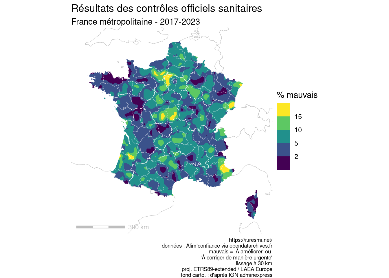
Can we see more in details? Using a 30 km kernel smoothing:
```{r}
#| label: fig-full-smooth
#| fig-cap: All controls (smoothed)
#| fig-alt: A map of bad controls in France (with kernel smoothing)
lissage_alim <- function(annee = NULL) {
  if (is.null(annee)) {
    alim <- alim |>
      filter(insee_dep < "97") |>
      mutate(poids = 1)

    annee_titre <- glue("{year(min(alim$date_inspection))}-{year(max(alim$date_inspection))}")
  } else {
    alim <- alim |>
      filter(insee_dep < "97",
             year(date_inspection) == annee) |>
      mutate(poids = 1)

    annee_titre <- annee
  }

  smooth_total <- alim |>
    lissage(poids, rayon, pixel, zone = fx)

  smooth_mauvais <- alim |>
    filter(synthese_eval_sanit %in% c("A améliorer", "A corriger de manière urgente")) |>
    lissage(poids, bandwidth = rayon, resolution = pixel, zone = fx)

  pcent_mauvais <- smooth_mauvais / smooth_total * 100

  raster::writeRaster(pcent_mauvais,
                    glue("results/alimconfiance_pcent_mauvais_{annee_titre}_fx.tif"),
                    overwrite = TRUE)

  p <- ggplot() +
    geom_sf(data = countries, color = "grey", fill = "white") +
    layer_spatial(as(pcent_mauvais, "SpatRaster")) +
    geom_sf(data = dep, fill = NA, color = "white", linewidth = .05) +
    geom_sf(data = reg_fx, fill = NA, color = "white", linewidth = .1) +
    scale_fill_viridis_b("% mauvais", breaks = c(2, 5, 10, 15), na.value = NA) +
    coord_sf(xlim = st_bbox(pcent_mauvais)[c(1, 3)],
             ylim = st_bbox(pcent_mauvais)[c(2, 4)],
             crs = proj_liss) +
    theme_void() +
    theme(plot.caption = element_text(size = 7))

  if (!is.null(annee)) {
    p +
      labs(title = glue("{annee_titre} - {format(nrow(alim), big.mark = ' ')} inspections"))
  } else {
    p +
      annotation_scale(height = unit(0.1, "cm"),
                       bar_cols = c("grey", "white"),
                       text_col = "grey",
                       line_col = "grey") +
      labs(title = "Résultats des contrôles officiels sanitaires",
           subtitle = glue("France métropolitaine - {annee_titre}"),
           caption = glue("https://r.iresmi.net/
                       données : Alim'confiance via opendatarchives.fr
                       mauvais = 'À améliorer' ou
                         'À corriger de manière urgente'
                       lissage à {rayon / 1000} km
                       proj. {nom_proj_liss}
                       fond carto. : d'après IGN adminexpress"))
  }
}

lissage_alim()
```
It confirms some hot-spots west of Paris, in Alsace, in Indre, Cher, Alpes-Maritimes and between Gironde and Landes. You are safer in Paris and Bretagne...
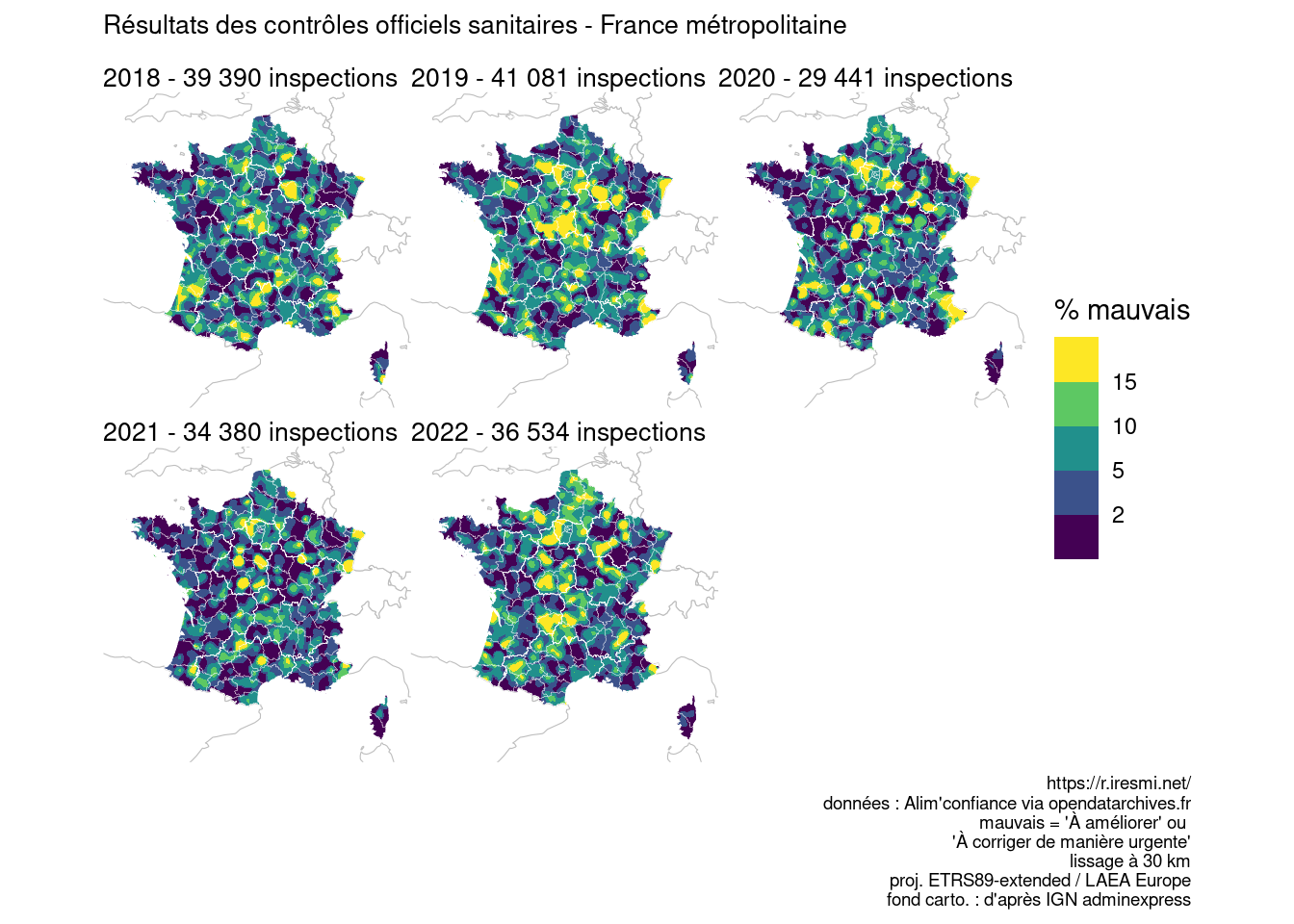
Has it changed?
```{r}
#| label: fig-periode
#| fig-cap: !expr 'glue("Evolution 2018-{year(max(alim$date_inspection)) - 1}")'
#| fig-alt: A small multiple map of bad controls in France (with kernel smoothing) by year
2018:(year(max(alim$date_inspection)) - 1) |>
  map(lissage_alim) |>
  reduce(`+`) +
  plot_layout(ncol = 3,
              guides = "collect") +
  plot_annotation(
    title = "Résultats des contrôles officiels sanitaires - France métropolitaine",
    caption = glue("https://r.iresmi.net/
                       données : Alim'confiance via opendatarchives.fr
                       mauvais = 'À améliorer' ou
                         'À corriger de manière urgente'
                       lissage à {rayon / 1000} km
                       proj. {nom_proj_liss}
                       fond carto. : d'après IGN adminexpress")) &
  theme(plot.caption = element_text(size = 7),
        plot.title =  element_text(size = 10))
```
No real trend...