library(Hmisc)
library(tidyverse)
library(RPostgreSQL)
library(glue)
library(httr)
library(rvest)
library(janitor)

cnx <- dbConnect(dbDriver("PostgreSQL"),
                 user = Sys.getenv("PG_IRESMI_USER"),
                 password = Sys.getenv("PG_IRESMI_PASS"),
                 host = Sys.getenv("PG_IRESMI_HOST"),
                 dbname = Sys.getenv("PG_IRESMI_DB"),
                 port = 5432
)Metadata are an essential part of a robust data science workflow ; they record the description of the tables and the meaning of each variable : its units, quality, allowed range, how we collect it, when it’s been recorded etc. Data without metadata are practically worthless. Here we will show how to transfer the metadata from PostgreSQL to R.
In PostgreSQL metadata can be stored in comments with the statements COMMENT ON TABLE ... IS '...' or COMMENT ON COLUMN ... IS '...'. So I hope your tables and columns have these nice comments and you can see them in psql or PgAdmin for example. But what about R ?
In R, metadata can be assigned as attributes of any object and mainly as « labels » for the columns. You may have seen labels when importing labelled data from SPSS for example.
We will use the {Hmisc} package which provides functions to manage labels. Another interesting package is {sjlabelled}.
We’ll start by adding a table and its metadata in PostgreSQL. I chose to use the list of all the french communes from the code officiel géographique (COG). The data is provided as a zipped CSV file ; luckily a data dictionary appears on the page so we’ll scrape it.
# data from https://www.insee.fr/fr/information/3720946

# download
dl <- tempfile()
GET("https://www.insee.fr/fr/statistiques/fichier/3720946/commune2019-csv.zip",
    write_disk(dl))
unzip(dl)

# import in PostgreSQL
read_csv("commune2019.csv",
         col_types = cols(.default = col_character())) %>%
  clean_names() %>%
  dbWriteTable(cnx, c("ref_cog", "commune2019"), ., row.names = FALSE)
dbSendQuery(cnx, "ALTER TABLE ref_cog.commune2019 ADD PRIMARY KEY (com, typecom);")

# get the data dictionary from INSEE
page <- GET("https://www.insee.fr/fr/information/3720946") %>%
  content()

table_info <- page %>%
  html_node("#titre-bloc-3 + div > p") %>%
  html_text() %>%
  str_trim() %>%
  str_replace_all("\\s+", " ")

columns_info <- page %>%
  html_node("table") %>%
  html_table() %>%
  clean_names() %>%
  mutate(designation_et_modalites_de_la_variable = str_trim(designation_et_modalites_de_la_variable),
         designation_et_modalites_de_la_variable = str_replace_all(designation_et_modalites_de_la_variable, "\\s+", " "),
         nom_de_la_variable = make_clean_names(nom_de_la_variable))

# add table metadata in PostgreSQL
dbSendQuery(cnx, glue_sql("COMMENT ON TABLE ref_cog.commune2019 IS {table_info}", .con = cnx))

# add columns metadata in PostgreSQL
walk2(columns_info$nom_de_la_variable,
      columns_info$designation_et_modalites_de_la_variable,
      ~ dbSendQuery(cnx, glue_sql("COMMENT ON COLUMN ref_cog.commune2019.{`.x`} IS {.y}", .con = cnx)))
Now we have this nice table:
=> \dt+ ref_cog.*
                                                      List of relations
 Schema  |    Name     | Type  |  Owner  |  Size   |                Description
---------+-------------+-------+---------+---------+-------------------------------------------------------------------
 ref_cog | commune2019 | table | xxxxxxx | 3936 kB | Liste des communes, arrondissements municipaux, communes déléguées et
                                                     communes associées au 1er janvier 2019, avec le code des niveaux
                                                     supérieurs (canton ou pseudo-canton, département, région)
(1 row)


=> \d+ ref_cog.commune2019
                                                      Table "ref_cog.commune2019"
  Column   | Type | Modifiers | Storage  | Stats target |                         Description
-----------+------+-----------+----------+--------------+----------------------------------------------------------------
 typecom   | text |           | extended |              | Type de commune
 com       | text |           | extended |              | Code commune
 reg       | text |           | extended |              | Code région
 dep       | text |           | extended |              | Code département
 arr       | text |           | extended |              | Code arrondissement
 tncc      | text |           | extended |              | Type de nom en clair
 ncc       | text |           | extended |              | Nom en clair (majuscules)
 nccenr    | text |           | extended |              | Nom en clair (typographie riche)
 libelle   | text |           | extended |              | Nom en clair (typographie riche) avec article
 can       | text |           | extended |              | Code canton. Pour les communes « multi-cantonales » code décliné
                                                            de 99 à 90 (pseudo-canton) ou de 89 à 80 (communes nouvelles)
 comparent | text |           | extended |              | Code de la commune parente pour les arrondissements municipaux et
                                                            les communes associées ou déléguées.
Indexes:
    "commune2019_pkey" PRIMARY KEY, btree (com, typecom)
Usually we query the data to R this way:
cog <- dbGetQuery(cnx,
"SELECT
  *
FROM ref_cog.commune2019
LIMIT 10")
We can create a function that will query the metadata of the table in information_schema.columns and add it to the data frame; the function expects a data frame, the name of the schema.table from which we get the comments and a connection handler. It will return the data frame with labels and an attribute metadata with the description of the table. We can also add a class to modify the default print method.
#' Add attributes to a dataframe from metadata read in the PostgreSQL database
#'
#' @param df (df) : a dataframe to which we'll add metadata
#' @param schema_table (char) : "schema.table" from which to read the comments
#' @param cnx (hdl) : a database connexion from RPostgreSQL::dbConnect()
#'
#' @return (df) : a dataframe with attributes
#'
#' @examples \dontrun{add_metadata(iris, "public.iris", cnx)}
add_metadata <- function(df, schema_table, cnx) {

  # get the table description and add it to a data frame attribute called "metadata"
  attr(df, "metadata") <- dbGetQuery(
    cnx,
    glue_sql("SELECT obj_description({schema_table}::regclass) AS table_description;",
             .con = cnx)) %>%
  pull(table_description)

  # get columns comments
  meta <- str_match(schema_table, "^(.*)\\.(.*)$") %>%
    glue_sql(
      "SELECT
        column_name,
        pg_catalog.col_description(
          format('%s.%s', isc.table_schema, isc.table_name)::regclass::oid,
                 isc.ordinal_position) AS column_description
      FROM information_schema.columns AS isc
      WHERE isc.table_schema = {s[2]}
        AND isc.table_name = {s[3]};",
      s = .,
      .con = cnx) %>%
    dbGetQuery(cnx, .)

  # match the columns comments to the variables
  label(df, self = FALSE) <- colnames(df) %>%
    enframe() %>%
    left_join(meta, by = c("value" = "column_name")) %>%
    pull(column_description)

  df <- as_tibble(df)
  class(df) <- c("meta", class(df))
  return(df)
}
The new print method for our meta-class:
#' Print a tibble of class "meta" where metadata have been added in a metadata
#' attribute
#'
#' @param x (tbl) : a tibble
#'
#' @return (tb) : the input tibble (invisibly)
print.meta <- function(x) {
  NextMethod(x)

  attr(x, "metadata") %>%
    cli::ansi_strwrap(simplify = FALSE) %>%
    paste("#", .) %>%
    pillar::style_subtle() %>%
    cat(sep = "\n")

  invisible(x)
}
Now we would do:
cog <- dbGetQuery(cnx,
  "SELECT
    *
  FROM ref_cog.commune2019
  LIMIT 100") %>%
  add_metadata("ref_cog.commune2019", cnx)
The table description is available with:
attr(cog, "metadata")[1] "Liste des communes, arrondissements municipaux, communes déléguées et communes associées au 1er janvier 2019, avec le code des niveaux supérieurs (canton ou pseudo-canton, département, région)"Or in the footer when we print the tibble:
cog# A tibble: 100 × 11
typecom com reg dep arr tncc ncc nccenr libelle can comparent
<labelled> <lab> <lab> <lab> <lab> <lab> <lab> <labe> <label> <lab> <labelle>
1 COM 01001 84 01 012 5 ABER… Aberg… L'Aber… 0108 <NA>
2 COM 01002 84 01 011 5 ABER… Aberg… L'Aber… 0101 <NA>
3 COM 01004 84 01 011 1 AMBE… Ambér… Ambéri… 0101 <NA>
4 COM 01005 84 01 012 1 AMBE… Ambér… Ambéri… 0122 <NA>
5 COM 01006 84 01 011 1 AMBL… Amblé… Ambléon 0104 <NA>
6 COM 01007 84 01 011 1 AMBR… Ambro… Ambron… 0101 <NA>
7 COM 01008 84 01 011 1 AMBU… Ambut… Ambutr… 0101 <NA>
8 COM 01009 84 01 011 1 ANDE… Ander… Andert… 0104 <NA>
9 COM 01010 84 01 011 1 ANGL… Angle… Anglef… 0110 <NA>
10 COM 01011 84 01 014 1 APRE… Aprem… Apremo… 0114 <NA>
# ℹ 90 more rows
# Liste des communes, arrondissements municipaux, communes déléguées et communes
# associées au 1er janvier 2019, avec le code des niveaux supérieurs (canton ou
# pseudo-canton, département, région)And you can see the metadata in the column headings of the RStudio viewer with View(cog):
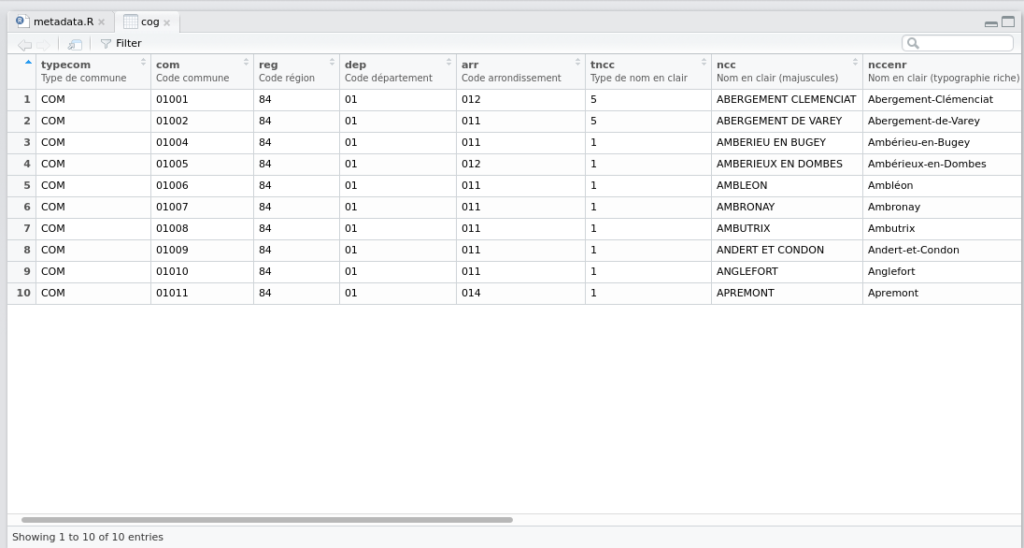
… the headings now show the metadata!
We can also use (not console-friendly):
contents(cog)
Data frame:cog  100 observations and 11 variables    Maximum # NAs:90

                                                                                                                                  Labels
typecom                                                                                                                  Type de commune
com                                                                                                                         Code commune
reg                                                                                                                          Code région
dep                                                                                                                     Code département
arr                                                                                                                  Code arrondissement
tncc                                                                                                                Type de nom en clair
ncc                                                                                                            Nom en clair (majuscules)
nccenr                                                                                                  Nom en clair (typographie riche)
libelle                                                                                    Nom en clair (typographie riche) avec article
can       Code canton. Pour les communes « multi-cantonales » code décliné de 99 à 90 (pseudo-canton) ou de 89 à 80 (communes nouvelles)
comparent                         Code de la commune parente pour les arrondissements municipaux et les communes associées ou déléguées.
              Class   Storage NAs
typecom   character character   0
com       character character   0
reg       character character   5
dep       character character   5
arr       character character   5
tncc      character character   0
ncc       character character   0
nccenr    character character   0
libelle   character character   0
can       character character   5
comparent character character  90
Or:
cog %>%
  label() %>%
  enframe()
# A tibble: 11 × 2
name value
<chr> <chr>
1 typecom Type de commune
2 com Code commune
3 reg Code région
4 dep Code département
5 arr Code arrondissement
6 tncc Type de nom en clair
7 ncc Nom en clair (majuscules)
8 nccenr Nom en clair (typographie riche)
9 libelle Nom en clair (typographie riche) avec article
10 can Code canton. Pour les communes « multi-cantonales » code décliné d…
11 comparent Code de la commune parente pour les arrondissements municipaux et …Or lastly, for one column:
label(cog$tncc)[1] "Type de nom en clair"We can also search for information in the variable names or in the labels with another function that can be helpful when we have a few hundred columns…
search_var <- function(df, keyword) {
  df %>%
    label() %>%
    enframe() %>%
    rename(variable = name,
           metadata = value) %>%
    filter_all(any_vars(str_detect(., regex(keyword, ignore_case = TRUE))))
}

search_var(cog, "canton")
# A tibble: 1 × 2
variable metadata
<chr> <chr>
1 can Code canton. Pour les communes « multi-cantonales » code décliné de …