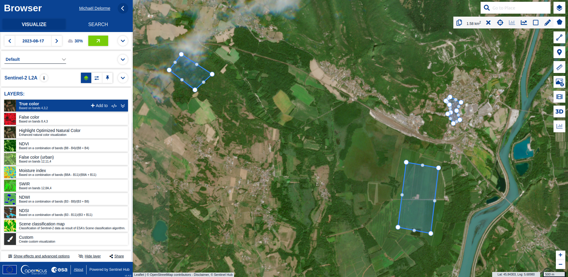
Copernicus OpenEO NDVI time series

The European Union has recently deployed a bunch of tools to access the data produced by the Copernicus Earth observation program: cool browser, APIs, Jupyter notebooks. Jupyter notebooks are cool: they allow to analyze satellite images without having to select, download, calibrate, mosaic gigaoctets of data on your own computer. But it’s Python! Hopefully the OpenEO API can now (since July 2023) be used from R and we can replicate one of the notebooks’ sample, also based on the documentation: creating a time serie of NDVI on different plots of land.

Sentinel-2 with the Copernicus Browser – 2023-08-17

Setup

Create an account on Copernicus first.

Install the required packages, including {openeo} to interact with the service. Then we can load them:

library(openeo) # OpenEO API implementation
library(signal) # optional, to filter the NDVI values at the end
library(tidyverse)
library(sf)
library(geojsonio) # converting the GIS data to GeoJSON
library(janitor)
library(fs)

Parameters

We draw 3 plots with QGIS for example. These plots are saved in a Geopackage plots.gpkg in WGS84. They will be converted to GeoJSON to be consumed by the API.

# 3 sample plots with field `landcover`: "agriculture", "forest", "city"
if (file_exists("plots.geojson")) file_delete("plots.geojson")

plots <- read_sf("plots.gpkg", layer = "plots") |> 
  write_sf("plots.geojson")

plots_json <- geojson_read("plots.geojson")

# temporal span (start - end)
date_span <- c("2020-01-01", "2022-12-31")

# Area name (for the final graphic plot)
location <- "Bugey"

Connect to API

cnx <- connect(host = "https://openeo.dataspace.copernicus.eu")

# Your console will require you to paste a code and your browser will ask to
# grant access
login()

Documentation about the resources

You can see the datasets and the processes available with a few commands.

list_collections()
describe_collection("SENTINEL2_L2A")

# List of available openEO processes with full metadata
processes <- list_processes()

# List of available openEO processes by identifiers (string)
print(names(processes))
process_viewer(processes)

# print metadata of the process with ID "load_collection"
print(processes$load_collection)

# get the formats
formats <- list_file_formats()

Initialize

Get the list of datasets and processing features available. We define some useful functions for the next part: NDVI computation, a mask to avoid clouds and the status of the batch job we’re about to construct and launch.

# get the collection list to get easier access to the collection ids, 
# via auto completion
collections <- list_collections()

# get the process collection to use the predefined processes of the back-end
p <- processes()

# compute NDVI
ndvi <- function(data, context) {
  red <- data[1]
  nir <- data[2]
  (nir - red) / (nir + red) 
}

# remove pixel not classified as vegetation (4) or non-vegetation (5), i.e.: water, 
# shadows, clouds, unclassified...
filter_unusable <- function(data, context) {
  scl <- data[3]
  !(scl == 4 | scl == 5)
}

# check processing status
status_job <- function(job) {
  while (TRUE) {
    if (!exists("started_at")) {
      started_at <- ymd_hms(job$created, tz = "UTC")
      message(capabilities()$title, "\n",
              "Job « ", job$description, " », ",
              "started on ", 
              format(started_at, tz = Sys.timezone(), usetz = TRUE), "\n")
    }
    
    current_status <- status(job)
    if (current_status == "finished") {
      message(current_status)
      break
    }
    
    current_duration <- seconds_to_period(difftime(Sys.time(),
                                                   started_at, 
                                                   units = "secs"))
    message(sprintf("%02d:%02d:%02d", 
                    current_duration@hour, 
                    minute(current_duration),
                    floor(second(current_duration))), " ",
            current_status, "...")
    Sys.sleep(30)
  }
}

Construct the batch job

That’s here that we use the NDVI computation to get the mean for each polygon at each date, using the mask.

s2_dataset <- p$load_collection(id = collections$SENTINEL2_L2A,
                            temporal_extent = date_span,
                            bands = c("B04", "B08", "SCL")) 

mask <- p$reduce_dimension(data = s2_dataset, 
                           dimension = "bands",
                           reducer = filter_unusable)

result <- s2_dataset |> 
  p$mask(mask) |> 
  p$reduce_dimension(dimension = "bands",
                     reducer = ndvi) |> 
  p$aggregate_spatial(geometries = plots_json, 
                      reducer = mean) |> 
  p$save_result(format = "CSV")

Launch and check job

It should take around 15 min…

job <- create_job(graph = result, 
                  title = "NDVI",
                  description = "NDVI plots")

start_job(job) 
# list_jobs() 
status_job(job)
# logs(job)

f <- download_results(job = job, folder = "results")

ndvi_data <- read_csv(f[[1]]) |>
  clean_names() 

That’s it! You have analysed at least 302 different scenes from the Sentinel-2 constellation !

Analyze

# filtering (optional)
ndvi_filtered <- ndvi_data |> 
  arrange(feature_index, date) |> 
  drop_na(avg_band_0) |> 
  group_by(feature_index) |> 
  mutate(ndvi = sgolayfilt(avg_band_0, n = 5)) |> 
  ungroup()

# plot
landcover_colors <- list("agriculture" = "goldenrod",
                         "forest" = "darkgreen",
                         "city" = "darkgrey")

ndvi_filtered |> 
  full_join(plots |> 
              st_drop_geometry() |> 
              mutate(feature_index = row_number() - 1)) |> 
  ggplot(aes(date, ndvi,
             group = landcover, 
             color = landcover,
             fill = landcover)) +
  geom_point(alpha = 0.2) +
  geom_smooth(span = 0.05) +
  scale_x_datetime(date_breaks = "year",
                   date_minor_breaks = "month",
                   date_labels = "%Y") +
  scale_y_continuous(breaks = scales::breaks_pretty()) +
  scale_color_manual(values = landcover_colors) +
  scale_fill_manual(values = landcover_colors) +
  guides(color = guide_legend(reverse = TRUE),
         fill = guide_legend(reverse = TRUE)) +
  labs(title = "Change of vegetation",
       subtitle = location,
       y = "NDVI",
       color = "Landcover", 
       fill = "Landcover")

ggsave("results/ndvi.png")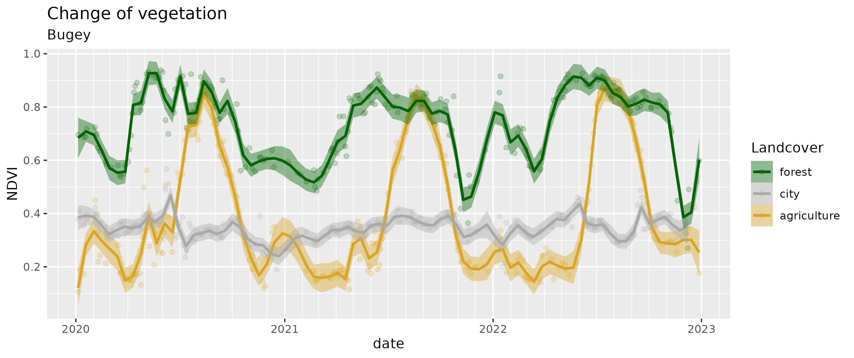

3 years of NDVI change in southern Jura

• The city stays relatively stable (mostly artifical) at 0.35;
• the deciduous forest shows the alternating seasons between 0.6 and 0.8;
• the corn fields show the growing seasons until the harvest from 0.2 to 0.8.

I still need to dig to replicate the mask convolution and the interpolation like in the Python notebook. Any tips?

Update: this post has been kindly presented by Edzer Pebesma at OpenGeoHub Summer school 2023. Yay!

Also cited in: https://github.com/r-spatial/discuss/issues/56#issuecomment-1742136917