library(tidyverse)
library(httr)
library(glue)
library(janitor)
library(jsonlite)
library(sf)

round_any <- function(x, accuracy, f = round) {
  f(x / accuracy) * accuracy
}
Great news! Météo-France has started to widen its open archive data. No API so far and a lot of files… What can we do?
We can start by selecting a few départements, here the 12 from Auvergne-Rhône-Alpes.
# which départements to download
sel_dep <- c("01", "03", "07", "15", "26", "38", "42", "43", "63", "69", "73", "74")

# for the map (code INSEE région)
sel_reg <- "84"
Scraping
Get some information about the available files for the daily data (Données climatologiques de base - quotidiennes).
# count files available
n_files <- GET("https://www.data.gouv.fr/api/2/datasets/6569b51ae64326786e4e8e1a/") |>
  content() |>
  pluck("resources", "total")

# get files informations
files_available <- GET(glue("https://www.data.gouv.fr/api/2/datasets/6569b51ae64326786e4e8e1a/resources/?page=1&page_size={n_files}&type=main")) |>
  content(as = "text", encoding = "UTF-8") |>
  fromJSON(flatten = TRUE) |>
  pluck("data") |>
  as_tibble(.name_repair = make_clean_names)
Download and open the files
if (!length(list.files("data"))) {
  files_available |>
    mutate(dep = str_extract(title, "(?<=departement_)[:alnum:]{2,3}(?=_)")) |>
    filter(dep %in% sel_dep,
           str_detect(title, "RR-T-Vent")) |>
    pwalk(\(url, title, format, ...) {
      GET(url,
          write_disk(glue("data/{title}.{format}"),
                     overwrite = TRUE))
          },
      .progress = TRUE)
}
We get 36 files…Each département has 3 files representing the recent years, 1950-2021 and before 1950.
# parsing problems with readr::read_delim
# we use read.delim instead
meteo <- list.files("data", pattern = ".*\\.csv.gz$", full.names = TRUE) |>
  map(read.delim,
      sep = ";",
      colClasses = c("NUM_POSTE" = "character",
                     "AAAAMMJJ" = "character"),
      .progress = TRUE) |>
  list_rbind() |>
  as_tibble(.name_repair = make_clean_names) |>
  mutate(num_poste = str_trim(num_poste),
         aaaammjj = ymd(aaaammjj))

# Map data
# See https://r.iresmi.net/posts/2021/simplifying_polygons_layers/
dep_sig <- read_sf("~/data/adminexpress/adminexpress_cog_simpl_000_2022.gpkg",
                   layer = "departement") |>
  filter(insee_reg == sel_reg) |>
  st_transform("EPSG:2154")
That’s a nice dataset of 19,254,143 rows!
Exploring
meteo |>
  summarise(.by= c(nom_usuel, num_poste, lat, lon),
            annee_max = max(year(aaaammjj))) |>
  mutate(statut = if_else(annee_max == year(Sys.Date()),
                          "active",
                          "inactive")) |>
  st_as_sf(coords = c("lon", "lat"), crs = "EPSG:4326") |>
  st_transform("EPSG:2154") |>
  ggplot() +
  geom_sf(data = dep_sig) +
  geom_sf(aes(color = statut,
              shape = statut),
          size = 2, alpha = 0.5) +
  scale_color_manual(values = c("inactive" = "chocolate4",
                                "active" = "chartreuse3")) +
  scale_shape_manual(values = c("inactive" = 16,
                                "active" = 17)) +
  labs(title = "Stations météo",
       subtitle = "Auvergne-Rhône-Alpes",
       caption = glue("données Météo-France (https://meteo.data.gouv.fr/)
                      fond carto d'après IGN Admin Express 2022
                      https://r.iresmi.net/ {Sys.Date()}")) +
  theme_minimal() +
  theme(plot.caption = element_text(size = 6))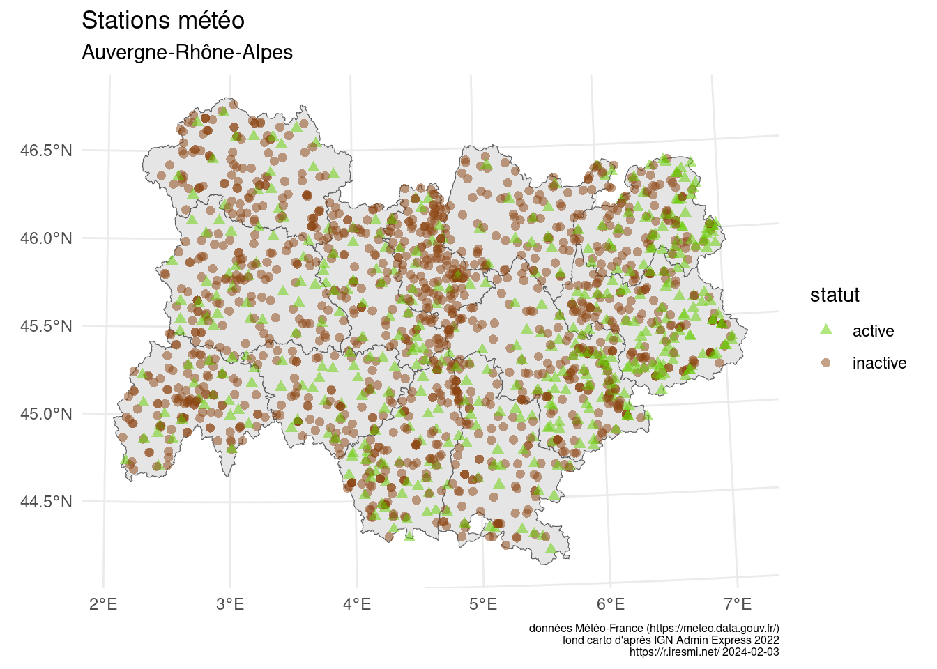
What would be an interesting station?
# longest temperature time series (possibly discontinuous)
meteo |>
  filter(!is.na(tx)) |>
  summarise(.by = c(nom_usuel, num_poste),
            deb = min(year(aaaammjj)),
            fin = max(year(aaaammjj)),
            n_annee = n_distinct(year(aaaammjj))) |>
  mutate(etendue = fin - deb) |>
  arrange(desc(n_annee))
# A tibble: 924 × 6
nom_usuel num_poste deb fin n_annee etendue
<chr> <chr> <dbl> <dbl> <int> <dbl>
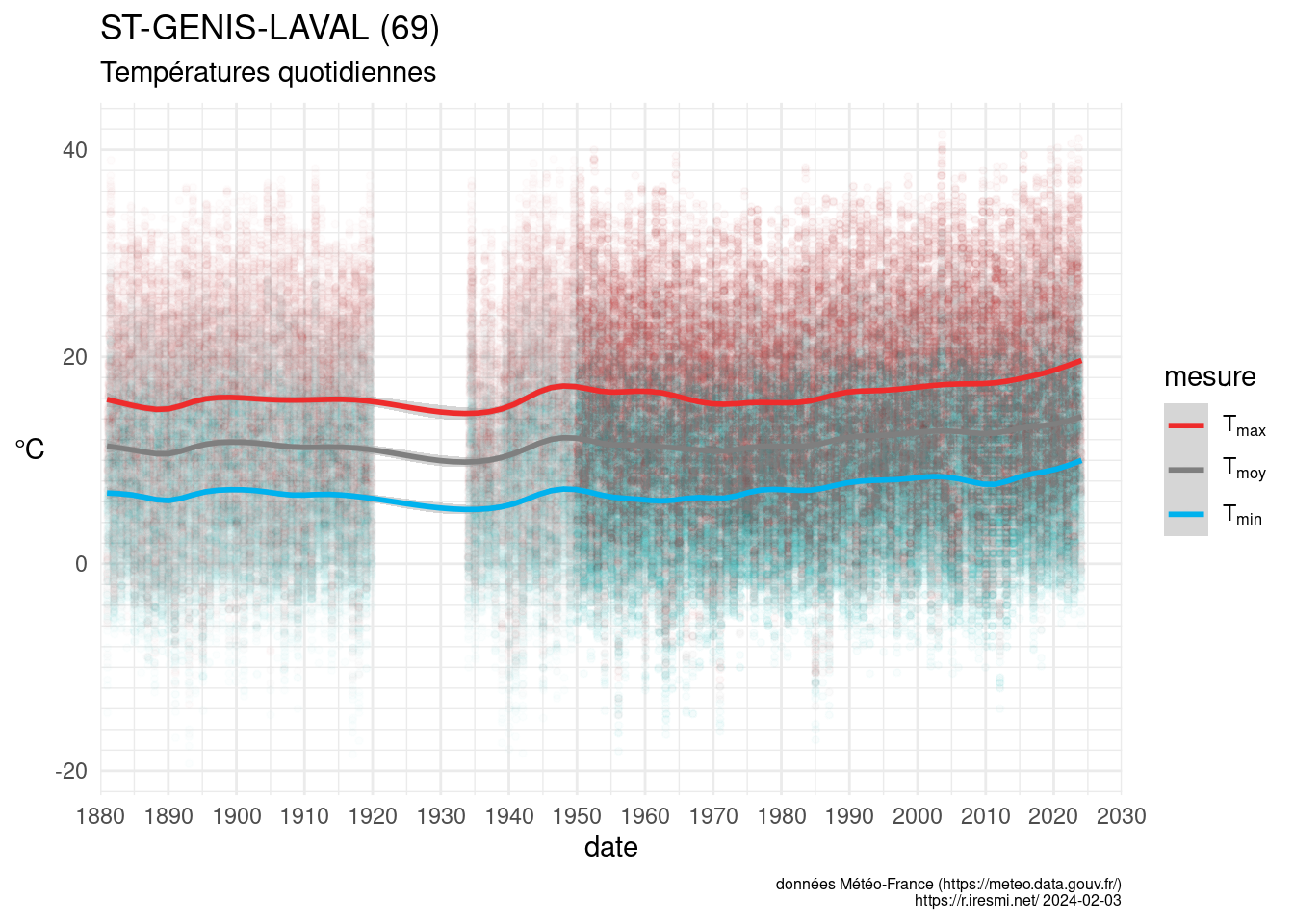
1 ST-GENIS-LAVAL 69204002 1881 2024 130 143
2 CHAMONIX 74056001 1880 2024 111 144
3 MONESTIER 38242001 1916 2024 108 108
4 MONTELIMAR 26198001 1920 2024 105 104
5 LYON-BRON 69029001 1920 2024 105 104
6 BOURG EN BRESSE 01053001 1890 1992 103 102
7 CLERMONT-FD 63113001 1923 2024 102 101
8 PRIVAS 07186002 1865 1968 98 103
9 LE PUY-CHADRAC 43046001 1928 2024 97 96
10 ANNECY 74010001 1876 1976 97 100
# ℹ 914 more rowsChoosing the longest time series:
meteo |>
  filter(num_poste == "69204002") |>
  mutate(tm = if_else(is.na(tm), (tx + tn) / 2, tm)) |>
  select(num_poste, nom_usuel, aaaammjj, tn, tm, tx) |>
  pivot_longer(c(tn, tm, tx),
               names_to = "mesure",
               values_to = "temp") |>
  mutate(mesure = factor(mesure,
                         levels = c("tx", "tm", "tn"))) %>% {
    ggplot(data = ., aes(aaaammjj, temp, color = mesure)) +
    geom_point(size = 1, alpha = 0.01) +
    geom_smooth(method = "gam",
                formula = y ~ s(x, bs = "cs", k = 30)) +
    scale_x_date(date_breaks = "10 years",
                 date_labels = "%Y",
                 expand = expansion(),
                 limits = ymd(paste0(c(
                   round_any(min(year(.$aaaammjj), na.rm = TRUE), 10, floor),
                   round_any(max(year(.$aaaammjj), na.rm = TRUE), 10, ceiling)), "0101"))) +
    scale_y_continuous(breaks = scales::breaks_pretty()) +
    scale_color_manual(values = c("tn" = "deepskyblue2",
                                  "tm" = "grey50",
                                  "tx" = "firebrick2"),
                       labels = list("tx" = bquote(T[max]),
                                     "tm" = bquote(T[moy]),
                                     "tn" = bquote(T[min]))) +
    labs(title = glue("{.$nom_usuel[[1]]} ({str_sub(.$num_poste[[1]], 1, 2)})"),
         subtitle = "Températures quotidiennes",
         x = "date",
         y = "℃",
         caption = glue("données Météo-France (https://meteo.data.gouv.fr/)
                        https://r.iresmi.net/ {Sys.Date()}")) +
    theme_minimal() +
    theme(plot.caption = element_text(size = 6),
          axis.title.y = element_text(angle = 0, vjust = 0.5))
  }