# Config ------------------------------------------------------------------

library(tidyverse)
library(elevatr)
library(sf)
# remotes::install_github("clauswilke/ggisoband")
library(ggisoband)
library(terra)
library(tidyterra)
library(glue)
library(janitor)
library(memoise)
library(magick)


# Parameters --------------------------------------------------------------

# Opentopo API
# Get a key on https://portal.opentopography.org/myopentopo
# elevatr::set_opentopo_key("xxx")


# Data --------------------------------------------------------------------

# Locations (decimal degrees, WGS84)
locations <- tribble(
  ~name,                     ~lon,       ~lat, ~alti, ~radius, ~iso_interval, ~zoom, ~source,
  "Aconcagua",         -70.017650, -32.658564,  6961,   10000,           150,    10,   "aws",
  "Эльбрус",            42.437876,  43.352404,  5643,   10000,           150,    10,   "aws",
  "Macizo Vinson",     -85.617388, -78.525399,  4892,   20000,           150,    10,   "aws",
  "Puncak Jaya",       137.158613,  -4.078606,  4884,   10000,           150,    10,   "aws",
  "Mount Kosciuszko",  148.263510, -36.455832,  2228,   15000,           100,    10,   "aws",
  "K2",                 76.513739,  35.881869,  8611,    5000,           180,    10,  "alos",
  )


# Area of interest --------------------------------------------------------

#' Create a {sf} layer from a point and radius
#'
#' @param lon (num) longitude (decimal degrees WGS84)
#' @param lat (num) latitude (decimal degrees WGS84)
#' @param radius (num) radius (meters)
#'
#' @return (sf) polygon
build_target <- function(lon, lat, radius) {
  tibble(x = lon,
         y = lat) |>
    st_as_sf(coords = c("x", "y"),
             crs = "EPSG:4326") |>
    st_buffer(radius) |>
    st_convex_hull()
}

#' Get elevation data
#'
#' @param target (sf) : area of interest
#' @param zoom (int) : zoom level ; z = 10 is good, z = 14 max resolution
#' @param source (char) : DEM source see {elevatr}. default "aws". "alos" is
#'   sometimes more detailed and with less artefacts but need an API key
#'
#' @return (data.frame) : with x, y, z coordinates
get_elevation <- memoise(
  function(target, zoom = 10, source = "aws") {
    get_elev_raster(target, z = zoom, src = source) |>
      rast() |>
      fortify() |>
      rename(z = 3)
  }
)

#' convert decimal degrees to DMS
#'
#' For displaying.
#' Note that we generally use (lon, lat) in computers, like (abscisse,
#' ordinates) or (x, y) but coordinates are generally displayed as "lat lon"
#'
#' @param coord (vector of num, length=2) : coordinates in decimal degrees :
#'   c(longitude, latitude)
#'
#' @return (char) : lat+lon coordinates : DD°MM′SS.SS″[NS] DDD°MM′SS.SS″[EW]
#'
#' @examples dec_to_sex(c(-155.468071, 19.820665))
dec_to_sex <- function(coord) {
  conv_dec_to_sex <- function(deg_dec, type) {
    deg <- abs(trunc(deg_dec))
    if (type == "lat" & deg > 90) {
      stop(glue("Latitude ({deg_dec}) shouldn't be over ±90°.
                   Did you mix latitude and longitude ?"))
    }
    if (type == "lon" & deg > 180) {
      stop(glue("Longitude ({deg_dec}) shouldn't be over ±180°.
                   Check your coordinates."))
    }
    min_dec <- (abs(deg_dec) - deg) * 60
    min <- trunc(min_dec)
    sec <- round(((min_dec - min) * 60), 2)
    h <- case_when(deg_dec < 0  & type == "lon" ~ "W",
                   deg_dec >= 0 & type == "lon" ~ "E",
                   deg_dec < 0  & type == "lat" ~ "S",
                   deg_dec >= 0 & type == "lat" ~ "N")
    sprintf("%02i°%02i′%.2f″%s", deg, min, sec, h)
  }
  glue("{conv_dec_to_sex(coord[2], type = 'lat')} {conv_dec_to_sex(coord[1], type = 'lon')}")
}


# Final plot --------------------------------------------------------------

#' Create a PNG (and its negative) of isolines around a place
#'
#' @param name (char) : place name
#' @param lon (num) : longitude (decimal degrees WGS84)
#' @param lat (num) : latitude (decimal degrees WGS84)
#' @param alti (num) : altitude (metres)
#' @param radius (num) : radius display range (metres)
#' @param iso_interval : elevation between isolines (metres)
#' @param zoom (int) : zoom level (1-14). default 10
#' @param source (char) : DEM source see {elevatr}. default "aws". "alos" is
#'   sometimes more detailed and with less artefacts but need an API key
#'
#' @return NULL (write on disk in the working directory)
#' @export
#'
#' @examples plot_isolines("Matterhorn", 7.658573, 45.976440, 4478, 5000, 100)
plot_isolines <- function(name, lon, lat, alti, radius, iso_interval,
                          zoom = 10, source = "aws") {

  target <- build_target(lon, lat, radius)
  target_bbox <- st_bbox(target)
  filename_image <- glue("{make_clean_names(name)}_{alti}_m")

  p <- get_elevation(target, zoom, source) |>
    ggplot() +
    geom_sf(data = target, fill = NA, color = NA) +
    geom_isobands(aes(x, y, z = z, fill = z),
                  binwidth = iso_interval, fill = NA) +
    coord_sf(xlim = target_bbox[c(1, 3)],
             ylim = target_bbox[c(2, 4)]) +
    labs(title = glue("{name} — {alti} m"),
         subtitle = dec_to_sex(c(lon, lat)),
         caption = "https://shirt.iresmi.net/") +
    theme_void() +
    theme(plot.title = element_text(family = "Arial narrow",
                                    face = "bold", size = 22),
          plot.title.position = "plot",
          plot.subtitle = element_text(family = "Arial narrow",
                                       face = "bold", size = 12),
          plot.caption = element_text(family = "Arial", size = 9))

  ggsave(glue("{filename_image}.png"), p,
         dpi = 300, width = 20, height = 20, units = "cm")

  # create negative image
  image_read(glue("{filename_image}.png")) |>
    image_negate() |>
    image_write(glue("{filename_image}_neg.png"))
}

locations |>
  pwalk(plot_isolines, .progress = TRUE)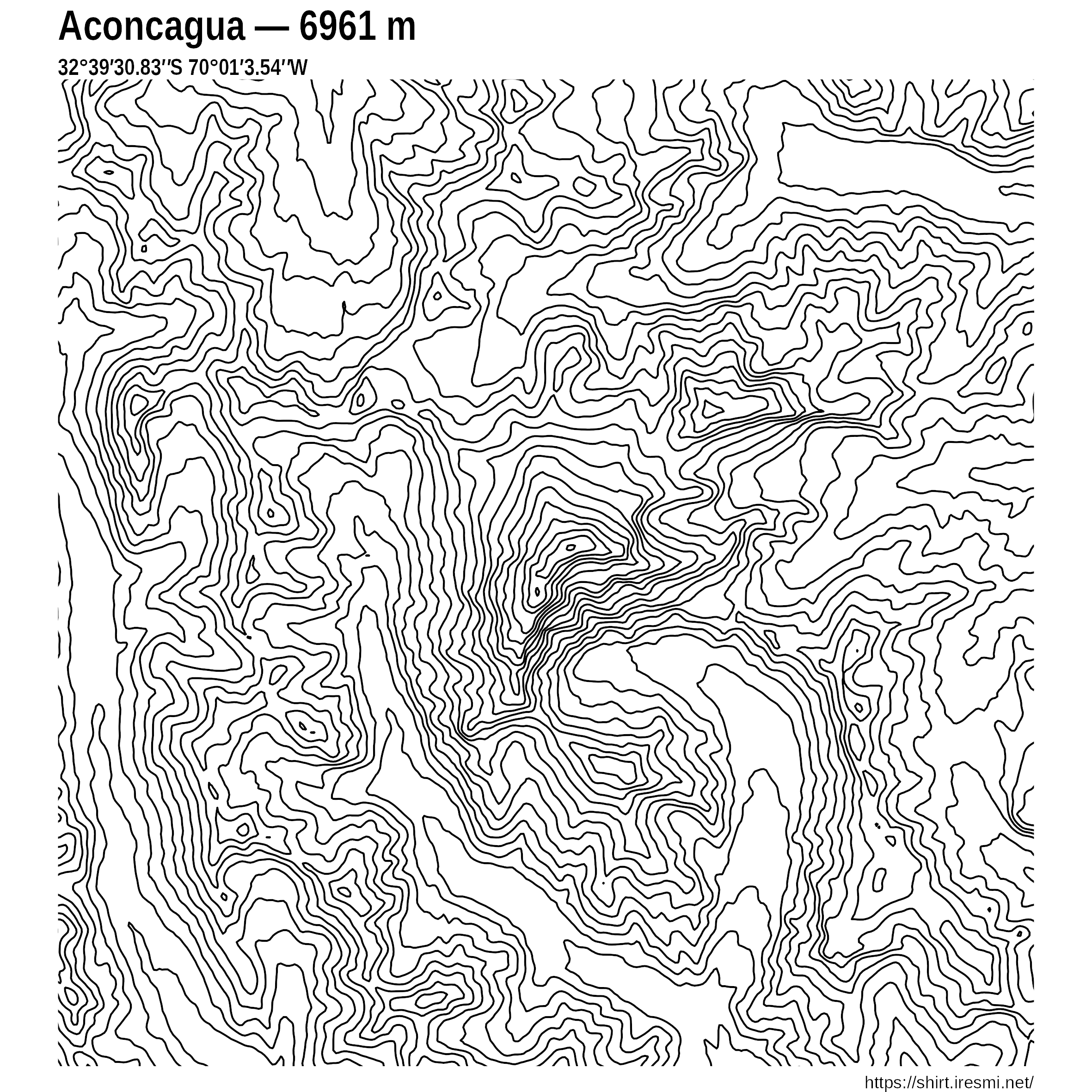
If you like mountains, R and T-shirts, I got you covered. Here we use {elevatr} to get a DEM around some well known summits and make a map consisting only of isohypses. It produces (sometimes) very nice visualizations.
And from these designs we can make nice T-shirts. You can buy some on https://shirt.iresmi.net/ and if your favorite mountain is not there, ask me and I’ll add it (or make it yourself, of course).
I intended to automate the process but sadly the Spreadshirt API doesn’t have an upload feature (!?). If you know a better shop, let me know…