Spatial autocorrelation

One in a Million – CC-BY-NC by Thomas Hawk

Day 29 of 30DayMapChallenge: « Population » (previously).

Setup

library(tidyverse)
library(sf)
library(glue)
library(sfdep)

Data

French administrative units (régions, départements, communes). Data is from an older post, based on IGN Admin Express.

# Keep only metropolitan France
com <- read_sf("~/data/adminexpress/adminexpress_cog_simpl_000_2022.gpkg",
               layer = "commune") |> 
  filter(insee_reg > "06") |> 
  st_transform("EPSG:2154") |> 
  mutate(densite = population / (surf_adminexpress_geo_ha / 100))

dep <- read_sf("~/data/adminexpress/adminexpress_cog_simpl_000_2022.gpkg", 
               layer = "departement_int") |> 
  st_transform("EPSG:2154") |> 
  st_join(com, left = FALSE)

reg <- read_sf("~/data/adminexpress/adminexpress_cog_simpl_000_2022.gpkg", 
               layer = "region_int") |> 
  st_transform("EPSG:2154") |> 
  st_join(com, left = FALSE)

Compute LISA

We will map the local indicators of spatial association (LISA) (Anselin 1995): high-high means that the spatial autocorrelation is positive and the local Moran indice is high; thus it also means that the population density of the commune is high in a cluster of high density communes.

lisa <- com |> 
  mutate(nb = st_contiguity(geom),
         wt = st_weights(nb, allow_zero = TRUE),
         lm = local_moran(densite, nb = nb, wt = wt, zero.policy = TRUE))

Map

lisa |> 
  unnest(lm) |> 
  mutate(in_cluster = if_else(p_folded_sim <= 0.1, mean, "n.s.")) |>
  drop_na(in_cluster) |> # get rid of off coast single communes (a few islands)
  ggplot() +
  geom_sf(aes(fill = in_cluster), color = NA, lwd = 0.2) +
  geom_sf(data = dep, linewidth = 0.05, color = "grey60") +
  geom_sf(data = reg, linewidth = 0.15, color = "grey50") +
  scale_fill_manual(values = c("red", "pink", "lightblue", "blue", "white")) +
  labs(title = "Population spatial autocorrelation",
       subtitle = "Metropolitan France",
       fill = "density",
       #color = "density",
       caption = glue("Data: based on IGN Admin Express 2022
                       https://r.iresmi.net/ {Sys.Date()}")) +
  theme_void() +
  theme(plot.caption = element_text(size = 6),
        plot.background = element_rect(fill = "black"),
        text = element_text(color = "white"))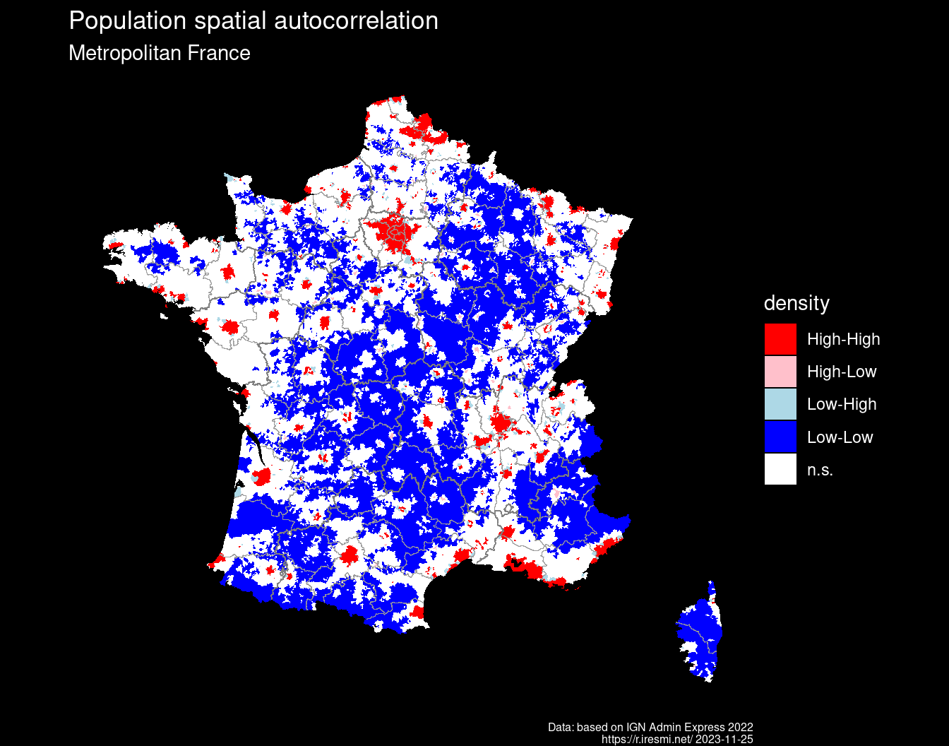

Figure 1: Population spatial autocorrelation

References

Anselin, Luc. 1995. “Local Indicators of Spatial Association—LISA.” Geographical Analysis 27 (2): 93–115. https://doi.org/10.1111/j.1538-4632.1995.tb00338.x.