library(sf)
library(ggplot2)
library(rnaturalearth)
library(glue)
library(terra)
library(ggspatial)

eqearth <- "EPSG:8857"

world <- ne_countries() |>
  st_transform(eqearth)

mask <- c(xmin = -179, ymin = -89, xmax = 179,  ymax = 89) |>
  st_bbox() |>
  st_as_sfc() |>
  st_set_crs("EPSG:4326") |>
  st_sf() |>
  st_segmentize(100) |>
  st_transform(eqearth)

acid_trend <- "global_omi_health_carbon_ph_trend_1985_P20230930.nc" |>
  rast() |>
  rotate() |>
  project(eqearth) |>
  mask(mask)
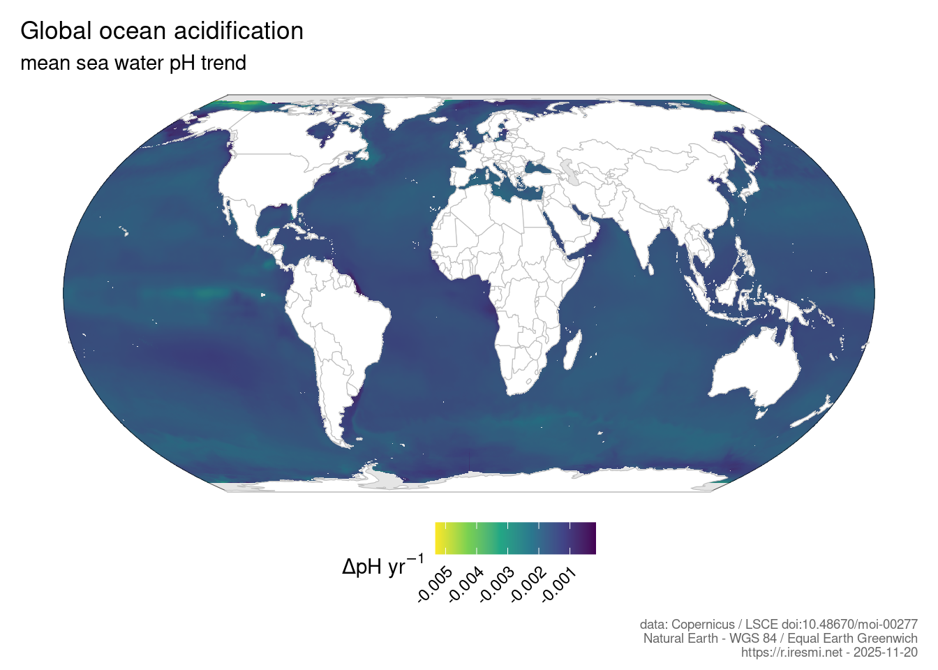
Day 20 of 30DayMapChallenge: « Water » (previously).
Global ocean acidification mean sea water pH trend map from Multi-Observations Reprocessing from Copernicus.
Data
Map
world |>
  ggplot() +
  layer_spatial(data = acid_trend,
                aes(fill = after_stat(band1))) +
  geom_sf(data = mask) +
  geom_sf(color = "grey", fill = "white") +
  scale_fill_viridis_c(name = bquote(Delta*pH~yr^-1),
                       direction = -1,
                       na.value = "white") +
  labs(title = "Global ocean acidification",
       subtitle = "mean sea water pH trend",
       caption = glue("data: Copernicus / LSCE doi:10.48670/moi-00277
                      Natural Earth - {st_crs(eqearth)$Name}
                      https://r.iresmi.net - {Sys.Date()}")) +
  theme_void() +
  theme(plot.caption = element_text(size = 7, color = "grey40"),
        plot.margin = unit(c(.2, .2, .2, .2), units = "cm"),
        legend.position = "bottom",
        legend.text = element_text(angle = 45, vjust = 1, hjust = 1))