Phoenician colonization

Figura de Astarté – Museo Arqueológico de Sevilla, Public domain, via Wikimedia Commons

I was reading Phoenician colonization from its origin to the 7th century BC (Manzano-Agugliaro et al. 2025) and thought it was an interesting dataset, but alas: it is split in four tables, behind a javascript redirect (wtf Taylor & Francis?) and with DMS coordinates (including typos and special characters)… So not easily reusable.

Let’s go build an accessible dataset.

Config

library(readr)
library(purrr)
library(dplyr)
library(stringr)
library(ggplot2)
library(forcats)
library(janitor)
library(sf)
library(rnaturalearth)
library(glue)
library(parzer)
library(leaflet)

sf_use_s2(FALSE)
knitr::knit_hooks$set(crop = knitr::hook_pdfcrop)

Data

We need to manually download the CSVs (parts 1, 2, 3 and 4) because there is an antiscraping mechanism… Then a little cleaning and coordinates parsing with the very nice {parzer} package let us build a spatial object with {sf}.

sources = list(
  c_10_bce = "data_raw/T0001-10.1080_17445647.2025.2528876.csv",
  c_09_bce = "data_raw/T0002-10.1080_17445647.2025.2528876.csv",
  c_08_bce = "data_raw/T0003-10.1080_17445647.2025.2528876.csv",
  c_07_bce = "data_raw/T0004-10.1080_17445647.2025.2528876.csv"
)

phoenician <- sources |> 
  imap(\(f, c) { read_csv(f) |>
         mutate(century_start_bce = parse_number(c))}) |> 
  list_rbind() |> 
  clean_names() |> 
  mutate(lon = parse_lon(str_replace(longitude_e, "−", "-")),
         lat = parse_lat(str_replace(latitude_n, ",", "."))) |> 
  st_as_sf(coords = c("lon", "lat"), crs = "EPSG:4326")

Maps

The resulting layer, mapped on a Natural Earth background, seems good.

world <- ne_countries() |> 
  st_intersection(phoenician |> 
                    st_bbox() |> 
                    st_as_sfc() |> 
                    st_buffer(4, joinStyle = "MITRE", mitreLimit = 10))

phoenician |> 
  ggplot() +
  geom_sf(data = world) +
  geom_sf(aes(color = fct_rev(as_factor(century_start_bce)))) +
  theme_void() +
  labs(title = "Phoenician colonies",
       subtitle = "10th c. BCE - 7th c. BCE",
       color = "from\n(century BCE)",
       caption = glue("data doi:10.1080/17445647.2025.2528876
                      https://r.iresmi.net/ {Sys.Date()}")) +
  theme_minimal() +
  theme(plot.caption = element_text(size = 6),
        plot.background = element_rect(fill = "white"))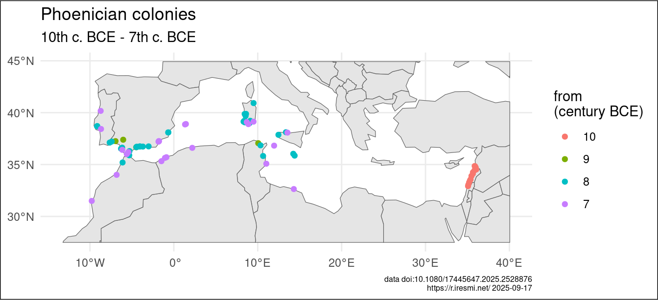

Figure 1: Phoenician colonies

You want more interactivity?
Using {leaflet}…

phoenician |> 
  leaflet() |> 
  addTiles(attribution = r"(
           <a href="https://r.iresmi.net/">r.iresmi.net</a>.
           data: Manzano-Agugliaro et al. 2025. doi:10.1080/17445647.2025.2528876;
           map: <a href="https://www.openstreetmap.org/copyright/">OpenStreetMap</a>)") |> 
  addCircleMarkers(popup = ~ glue("<b>{settlement}</b><br /><br />
                                  from {century_start_bce}th c. BCE \\
                                  {if_else(!is.na(centuries_of_subsequent_permanence), 
                                  paste0('<br />to ', centuries_of_subsequent_permanence), '')}"),
                   clusterOptions = markerClusterOptions())

Figure 2: Phoenician colonies (interactive)

Export

We can build a clean GIS data layer using the Geopackage format (and a CSV just in case):

phoenician |> 
  st_write(
    "data/phoenician_settlements.gpkg",
    layer = "phoenician_settlements",
    layer_options = c(
      "IDENTIFIER=Phoenician colonization from its origin to the 7th century BC",
      glue("DESCRIPTION=Data from: 
            Manzano-Agugliaro, F., Marín-Buzón, C., Carpintero-Lozano, S., & López-Castro, J. L. (2025). \\
            Phoenician colonization from its origin to the 7th century BC. Journal of Maps, 21(1). \\
            https://doi.org/10.1080/17445647.2025.2528876
           
            Available on https://doi.org/10.5281/zenodo.17141060
           
            Extracted on {Sys.Date()} – https://r.iresmi.net/posts/2025/phoenician")),
    delete_layer = TRUE, 
    quiet = TRUE)

phoenician |> 
  select(-c(latitude_n, longitude_e)) |> 
  bind_cols(st_coordinates(phoenician)) |> 
  rename(lon_wgs84 = X,
         lat_wgs84 = Y) |> 
  st_drop_geometry() |> 
  write_csv("data/phoenician_settlements.csv")

And lastly we store them in a public repository; they are now available on Zenodo and therefore even have a doi:10.5281/zenodo.17141060

References

Manzano-Agugliaro, Francisco, Carmen Marín-Buzón, Susana Carpintero-Lozano, and José Luis López-Castro. 2025. “Phoenician Colonization from Its Origin to the 7th Century BC.” Journal of Maps 21 (1): 2528876. https://doi.org/10.1080/17445647.2025.2528876.