# Carto décès COVID 19 hexagones
# France métro. + DOM
# Animation
# DONNEES SPF

# packages ----------------------------------------------------------------
library(tidyverse)
library(httr)
library(fs)
library(sf)
library(readxl)
library(janitor)
library(glue)
library(tmap)
library(grid)
library(classInt)
library(magick)
library(geogrid)


# sources -----------------------------------------------------------------

# https://www.data.gouv.fr/fr/datasets/donnees-hospitalieres-relatives-a-lepidemie-de-covid-19/
fichier_covid <- "donnees/covid.csv"
url_donnees_covid <- "https://www.data.gouv.fr/fr/datasets/r/63352e38-d353-4b54-bfd1-f1b3ee1cabd7"

# https://www.insee.fr/fr/statistiques/2012713#tableau-TCRD_004_tab1_departements
fichier_pop <- "donnees/pop.xlsx"
url_donnees_pop <- "https://www.insee.fr/fr/statistiques/fichier/2012713/TCRD_004.xlsx"

# Adminexpress : à télécharger manuellement
# https://geoservices.ign.fr/documentation/diffusion/telechargement-donnees-libres.html#admin-express
aex <- path_expand("~/data/adminexpress/adminexpress_cog_simpl_000_2022.gpkg")


# config ------------------------------------------------------------------

force_download <- FALSE # retélécharger même si le fichier existe et a été téléchargé aujourd'hui ?


# téléchargement ------------------------------------------------------

dir_create("donnees")
dir_create("resultats")
dir_create("resultats/animation_spf_hex")

if (!file_exists(fichier_covid) |
    file_info(fichier_covid)$modification_time < Sys.Date() |
    force_download) {
  GET(url_donnees_covid,
      progress(),
      write_disk(fichier_covid, overwrite = TRUE)) |>
    stop_for_status()
}

if (!file_exists(fichier_pop)) {
  GET(url_donnees_pop,
      progress(),
      write_disk(fichier_pop)) |>
    stop_for_status()
}


# données -----------------------------------------------------------------

covid <- read_csv2(fichier_covid) |>
  filter(jour < "2020-05-26")

# adminexpress prétéléchargé
dep <- read_sf(aex, layer = "departement") |>
  filter(insee_dep < "971") |>
  st_transform("EPSG:2154") |>
  mutate(surf_ha = st_area(geom) * 10000)

# grille hexagonale
dep_cells_hex <- calculate_grid(shape = dep, grid_type = "hexagonal", seed = 1)
dep_hex <- assign_polygons(dep, dep_cells_hex)

# Pour les DOM on duplique et déplace un département existant
d971 <- dep_hex[dep_hex$insee_dep == "29", ]
d971$geometry[[1]] <- d971$geometry[[1]] + st_point(c(0, -150000))
d971$insee_dep <- "971"

d972 <- dep_hex[dep_hex$insee_dep == "29", ]
d972$geometry[[1]] <- d972$geometry[[1]] + st_point(c(0, -250000))
d972$insee_dep <- "972"

d973 <- dep_hex[dep_hex$insee_dep == "29", ]
d973$geometry[[1]] <- d973$geometry[[1]] + st_point(c(0, -350000))
d973$insee_dep <- "973"

d974 <- dep_hex[dep_hex$insee_dep == "2A", ]
d974$geometry[[1]] <- d974$geometry[[1]] + st_point(c(0, 250000))
d974$insee_dep <- "974"

d976 <- dep_hex[dep_hex$insee_dep == "2A", ]
d976$geometry[[1]] <- d976$geometry[[1]] + st_point(c(0, 350000))
d976$insee_dep <- "976"

dep_hex <- bind_rows(dep_hex, d971, d972, d973, d974, d976)

# population
pop <- read_xlsx(fichier_pop, skip = 2) |>
  clean_names() |>
  select(insee_dep = x1,
         x2020)

# lignes de séparation DOM / métropole
encarts <- st_multilinestring(
  list(st_linestring(matrix(c(1100000, 6500000,
                              1100000, 6257000,
                              1240000, 6257000), byrow = TRUE, nrow = 3)),
       st_linestring(matrix(c(230000, 6692000,
                              230000, 6391000), byrow = TRUE, nrow = 2)))) |>
  st_sfc() |>
  st_sf(id = 1, geometry = _) |>
  st_set_crs("EPSG:2154")


# traitement --------------------------------------------------------------

# jointures des données
creer_df <- function(territoire, date = NULL) {
  territoire |>
    left_join(pop, join_by(insee_dep)) |>
    left_join(
      covid |>
        filter(jour == ifelse(is.null(date), max(jour), date),
               sexe == 0) |>
        rename(deces = dc,
               reanim = rea,
               hospit = hosp),
      join_by(insee_dep == dep)) |>
    mutate(incidence = deces / x2020 * 1e5)
}

incidence <- creer_df(dep_hex)

set.seed(1234)
classes <- classIntervals(incidence$incidence, n = 6, style = "kmeans", dataPrecision = 0)$brks

# carto -------------------------------------------------------------------
# décès cate du dernier jour dispo

carte <- tm_layout(title = glue("COVID-19\nFrance\n{max(covid$jour)}"),
                         legend.position = c("left", "bottom"),
                         frame = FALSE) +
  tm_shape(incidence) +
  tm_polygons(col = "incidence", title = "décés\ncumulés pour\n100 000 hab.",
              breaks = classes,
              palette = "viridis",
              legend.reverse = TRUE,
              legend.format = list(text.separator = "à moins de",
                                   digits = 0)) +
  tm_text("insee_dep", size = .8) +
  tm_shape(encarts) +
  tm_lines(lty = 3) +
  tm_credits(glue("http://r.iresmi.net/
                    classif. kmeans
                    données départementales Santé Publique France,
                    INSEE RP 2020, d'après IGN Adminexpress 2020"),
             position = c(.6, 0),
             size = .5)

fichier_carto <- glue("resultats/covid_hex_fr_{max(covid$jour)}.png")

tmap_save(carte, fichier_carto, width = 900, height = 900, scale = .4)


# animation ---------------------------------------------------------------

image_animation <- function(date) {
  message(glue("\n\n{date}\n==========\n"))

  m <- creer_df(dep_hex, date) |>
    tm_shape() +
    tm_polygons(col = "incidence", title = "décés\ncumulés pour\n100 000 hab.",
                breaks = classes,
                palette = "viridis",
                legend.reverse = TRUE,
                legend.format = list(text.separator = "à moins de",
                                     digits = 0)) +
    tm_text("insee_dep", size = .8) +
    tm_shape(encarts) +
    tm_lines(lty = 3) +
    tm_layout(title = glue("COVID-19\nFrance\n{date}"),
              legend.position = c("left", "bottom"),
              frame = FALSE) +
    tm_credits(glue("http://r.iresmi.net/
                    classif. kmeans
                    données départementales Santé Publique France,
                    INSEE RP 2020, d'après IGN Adminexpress 2020"),
               position = c(.6, 0),
               size = .5)

  tmap_save(m, glue("resultats/animation_spf_hex/covid_fr_{date}.png"),
            width = 800, height = 800, scale = .4,)
}

unique(covid$jour) |>
  walk(image_animation)

animation <- glue("resultats/deces_covid19_fr_hex_spf_{max(covid$jour)}.gif")

dir_ls("resultats/animation_spf_hex") |>
  map(image_read) |>
  image_join() |>
  image_animate(fps = 2, optimize = TRUE) |>
image_write(animation)The départements are the second level of administrative government in France. They neither have the same area nor the same population and this heterogeneity provides a few challenges for a fair and accurate map representation (see the post on smoothing).
However if we are just interested in the départements as units, we can use a regular grid for visualization. Since France is often called the hexagon, we could even use an hexagon tiling (a fractal map !)…
Creating the grid and conserving minimal topological relations and the general shape can be time consuming, but thanks to Geogrid it’s quite easy. The geogrid dev page provides nice examples. We will reuse our code of the COVID19 animation. The resulting GIS file is provided below.
The global shape and relations are well rendered. Deformations are quite important for the small départements around Paris, but the map remains legible.
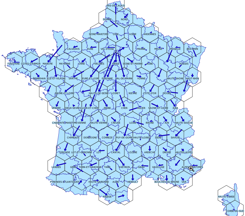
Get the resulting file (geopackage), in EPSG:2154 (Lambert93)