Flow

Flow – CC-BY-NC by Sebastian Bender

Day 17 of 30DayMapChallenge: « Flow » (previously).

Mapping the commuters to Lyon in France. Data comes from INSEE and is part of the national census.

Setup

library(tidyverse)
library(sf)
library(glue)
library(janitor)

Data

Paris, Lyon and Marseille are subdivided in this dataset (by arrondissement); we filter out Lyon origins and keep only Lyon destinations and we aggregate the arrondissements for the 3 cities.

# Home-work commute in France 2019, by commune
# https://www.insee.fr/fr/information/2383337
# https://www.insee.fr/fr/statistiques/6454112
hwc_file <- "base-csv-flux-mobilite-domicile-lieu-travail-2019.zip"

if (!file.exists(hwc_file)) {
  download.file(paste0("https://www.insee.fr/fr/statistiques/fichier/6454112/",
                       hwc_file), 
                hwc_file)
}

hwc <- read_delim(hwc_file,
                  delim = ";",
                  locale = locale(decimal_mark = ".")) |> 
  clean_names() |> 
  filter(str_detect(dclt, "6938[1-9]"),
         !str_detect(codgeo, "6938[1-9]")) |> 
  mutate(across(c(codgeo, dclt), 
                ~ case_when(between(.x, "13201", "13216") ~ "13055",
                            between(.x, "75101", "75120") ~ "75056",
                            between(.x, "69381", "69389") ~ "69123",
                            .default = .x))) |> 
  group_by(codgeo, dclt) |> 
  summarise(nbflux_c19_actocc15p = sum(nbflux_c19_actocc15p),
            .groups = "drop")

# France communes and régions (polygons)
# See https://r.iresmi.net/posts/2021/simplifying_polygons_layers/ for the data
c("commune", "region") |> 
  set_names() |> 
  map(\(x) read_sf("~/data/adminexpress/adminexpress_cog_simpl_000_2022.gpkg",
                   layer = x) |> 
        filter(insee_reg > "06") |> 
        st_transform("EPSG:2154")) |> 
  list2env(envir = .GlobalEnv)

Build flow coordinates

# get coordinates for origin points
com_orig <- commune |> 
  st_point_on_surface() |> 
  mutate(x = st_coordinates(geom)[, 1],
         y = st_coordinates(geom)[, 2]) |> 
  select(insee_com, x, y)

# we only need one destination point: Lyon
com_dest <- com_orig |> 
  filter(insee_com == "69123")

# Add origine and destination coords to the commute table
flow <- hwc |> 
  left_join(com_orig, 
            join_by(codgeo == insee_com)) |> 
  left_join(com_dest, 
            join_by(dclt == insee_com), 
            suffix = c("_orig", "_dest")) 

Map

ggplot(region) +
  geom_sf(color = "grey70",
          fill="grey95") +
  geom_curve(data = flow,
             aes(x = x_orig, y = y_orig, xend = x_dest, yend = y_dest,
                 linewidth = nbflux_c19_actocc15p, 
                 alpha = nbflux_c19_actocc15p),
             color = "dodgerblue3",
             curvature = 0.2) +
  scale_linewidth_continuous(labels = scales::label_number(big.mark = " "),
                             trans = "log10",
                             breaks = c(10, 100, 1000, 10000),
                             range = c(0.05, 3)) +
  scale_alpha_continuous(labels = scales::label_number(big.mark = " "),
                         trans = "log10",
                         breaks = c(10, 100, 1000, 10000),
                         range = c(0.05, .4)) +
  labs(title = "Working flow to Lyon",
       subtitle = "2019",
       linewidth = "workers",
       alpha = "workers",
       caption = glue("https://www.iresmi.net {Sys.Date()}
                      Base map from IGN Admin Express 2022
                      Data: INSEE 2019")) +
  theme_void() +
  theme(text = element_text(family = "Courier"),
        plot.margin = margin(0, .3, 0.1, .3, "cm"),
        plot.background = element_rect(color = NA, fill = "white"),
        plot.caption = element_text(size = 6))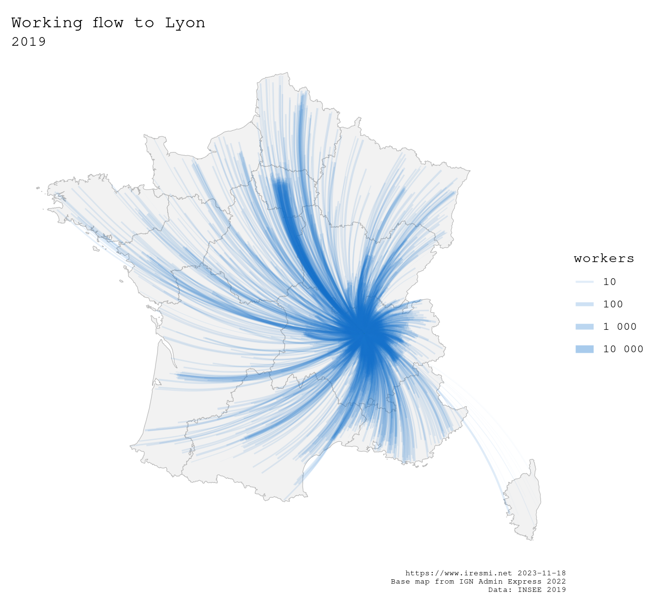

Figure 1: Working in Lyon

The 2-hours commute from Paris by TGV seems popular…